Before introducing computational apparatus for limits, we need to finish the definitions by defining some variations: one-sided limits, limits at infinity and "limits" of infinity (which are in quotes because technically they are not limits at all).
Change the definition so that \(f(x) \) is only required to approach \(L\) when \(x \to a \) if \(x \) is greater than \(a \text{.}\) We say \(x \) "approaches \(a \) from the right," thinking of a number line. If the value of \(f(x) \) approaches \(L \) when \(x \) approaches \(a \) from the right, we say that the limit from the right of \(f(x) \) at \(x=a \) is \(L \text{,}\) and denote this \(\displaystyle\lim_{x \to a^+} f(x) = L \text{.}\) If we require \(f(x) \) to approach \(L \) when \(x \) approaches \(a \) but only for those \(x \) that are less than \(a \text{,}\) this is called having a limit from the left and is denoted \(\displaystyle\lim_{x \to a^-}
f(x) = L \text{.}\)
Just like wind directions (North wind, South wind, etc.), one-sided limits are named for the direction they come from, not the direction \(x \) is moving. Thus, \(\displaystyle\lim_{x \to 0^+} \) is evaluated by letting \(x \) approch zero from the positive direction, as shown to the right.
Both kinds of one-sided limits require something less stringent, so the statement \(\displaystyle\lim_{x \to a} f(x) = L \) automatically implies both \(\displaystyle\lim_{x \to a^+} f(x) = L \) and \(\displaystyle\lim_{x \to a^-} f(x) = L \text{.}\) Likewise, if \(f(x) \) is forced to approach \(L \) when \(x \) approaches \(a\) from the right, but also when \(x \) approaches \(a \) from the left, then this covers all \(x \text{,}\) and the (unrestricted) limit will be \(L \text{.}\) If you want, you can summarize this as a theorem -- wait, no it’s too puny, let’s make it a proposition. We won’t be referring to this too often, but here it is.
For every function \(f \) and real numbers \(a \) and \(L \text{,}\)
\begin{equation*}
\displaystyle\lim_{x \to a} f(x) = L \text{ if and only if }
\lim_{x \to a^+} f(x) = L \text{ and } \lim_{x \to a^-} f(x) = L \, .
\end{equation*}
In words, a limiting value for a function exists at a point if and only if the two one-sided limits exist are are equal.
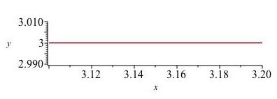
Let \(f(x) = \lfloor x \rfloor \text{,}\) the greatest integer function. Let’s evaluate the one-sided limits and two-sided limit at a couple of values. First, take \(a = \pi \text{,}\) you know, the irrational number beginning \(3.14\ldots \text{.}\) If we just look near this value, say between \(3.1 \) and \(3.2 \text{,}\) it is completely flat: a constant function, taking the value 3 everywhere. So of course the limit at \(x=\pi \) will also be 3. This is the same by words or pictures; see Figure 2.9.
By the formal definition, no matter what \(\varepsilon \) is chosen, you can take \(\delta = 0.1 \text{,}\) say, and \(f(x) \) will be within \(\varepsilon \) of 3 because it will be exactly 3. So the limit is 3, hence so are both one-sided limits as in the picture just above.
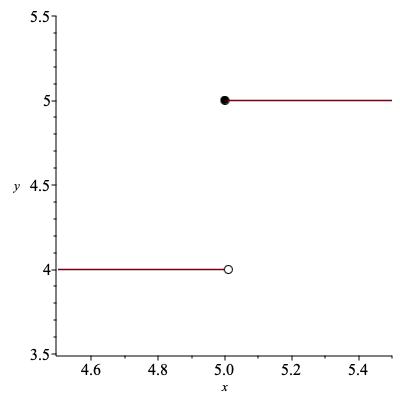
Now take \(x \) to be an integer, say \(a=5 \text{.}\) The limit from the right looks like it did before, with \(f(x) \) taking the value 5 for every sufficiently close \(x \) (here sufficient means within 1) greater than 5. On the other hand, when \(x \) is close to 5 but less than 5, we will have \(f(x) = 4 \text{,}\) as in the picture below. Thus,
You have already seen the pictorial and verbal version of a limit at infinity. Here is the formal definition. It repeats a lot of the definition of a limit at \(x=a \text{.}\) The only difference is that instead of having to come up with an interval \((a-\delta , a+\delta)\) guaranteeing \(f(x) \) is within \(\varepsilon \) of the limit, you have to come up with an "interval near infinity". This turns out to mean an interval \((M,\infty) \text{.}\) In other words, there must be a real number \(M \) guaranteeing \(f(x) \) is within \(\varepsilon \) of \(L \) when \(x \gt M \text{.}\)
Informally, "close to infinity" turns into "sufficiently large". In the tolerance/accuracy analogy, getting \(f(x) \) to be close to \(L\) to within the acceptable tolerance will result from guaranteed largeness of the input rather than guaranteed closeness to \(a \text{.}\)
For any positive real number \(\varepsilon \) (think of this as acceptable tolerance in the \(y \) value) there is a corresponding real \(M\) (think of this as guaranteed minimum value for \(x\)) such that for any \(x \) greater than \(M \text{,}\)\(f(x) \) is guaranteed to be in the interval \((L - \varepsilon , L + \varepsilon) \text{.}\)
If a real number \(L \) exists satisfying this, we write \(\displaystyle\lim_{x \to \infty}
f(x) = L \text{.}\) Sometimes to be completely unambiguous, we put in a plus sign: \(\displaystyle\lim_{x \to +\infty} f(x) = L \text{.}\)
Limits at \(-\infty \) are defined exactly the same except for a single inequality that is reversed. Now the implication that must hold is that for some (possibly very negative) \(M \text{,}\)
\begin{equation*}
x \lt M \Longrightarrow |f(x) - L| \lt \varepsilon \, .
\end{equation*}
When this holds, we write \(\displaystyle\lim_{x \to -\infty} f(x) = L \text{.}\) When no such \(L \) exists, we write \(\displaystyle\lim_{x \to -\infty} f(x) \) does not exist.
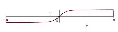
Let \(f(x) := \frac{x}{\sqrt{1+x^2}} \text{.}\) Because \(\sqrt{1+x^2} \) is a little bigger than \(|x| \) but almost the same when \(x \) or \(-x \) is large, this function satisfies
The graph of this function is shown in Figure 2.14. It has horizontal asymptotes at 1 and \(-1 \text{.}\) This suggests how to define a horizontal asymptote.
A function \(f \) or its graph is said to have a horizontal asymptote at height \(b \) if \(\displaystyle\lim_{x \to \infty} f(x) = b \) or \(\displaystyle\lim_{x \to - \infty} f(x) = b \text{.}\)
Sketch a graph of a function \(f \) for which \(\displaystyle\lim_{x \to -\infty} f(x) \) exists but \(\displaystyle\lim_{x \to +\infty} f(x) \) does not.
Give a formula defining a function \(g(x) := \cdots \) such that \(\displaystyle\lim_{x \to -\infty} g(x) \) exists but \(\displaystyle\lim_{x \to +\infty} g(x) \) does not.
Consider the function \(f(x) = 1/x^2 \text{,}\) defined for all real numbers except zero. What happens to \(f(x) \) as \(x \to 0 \) ? By our definitions, \(\displaystyle\lim_{x \to 0} 1/x^2 \) does not exist. But we can see that \(f(x) \) "goes to infinity". Because infinity is not a number, the limit technically does not exist. However, it is useful to classify limits which don’t exist as ones where the function approaches \(\infty \) (or \(-\infty\)) versus ones where there is no consistent behavior.
This time, instead of staying within a tolerance of \(\varepsilon \) in the output, we make the output sufficiently large (greater than any given \(N\)) or small. We do this by guaranteeing \(\delta \) accuracy in the input (for limits as \(x \to a\)) or by making the input sufficiently large or small (limits as \(x \to \pm \infty\)).
If \(f \) is a function and \(a \) is a real number, we say that \(\displaystyle\lim_{x \to a} f(x) = +\infty \) if for every real \(N \) there is a \(\delta \gt 0 \) such that \(0 \lt \left\lvert x-a\right\rvert \lt \delta \) implies \(f(x) \gt N \text{.}\)
Again, if we reverse the last inquality to require that \(f(x) \lt N\) (and \(N \) can be a very negative number) we get the definition for a limit of negative infinity. Please remember these are all subcases of limits that don’t exist! If you show that a limit is infinity, you have shown that the limit does not exist (and you have specified a particular reason it doesn’t exist).
Let’s check that \(\displaystyle\lim_{x \to 0} 1/x^2 = +\infty \text{.}\) Given a positive real number \(N \text{,}\) how can we ensure \(f(x) \gt N\text{?}\)
Answer: for positive numbers, \(f \) is decreasing and \(f(x) = N\) precisely when \(x = 1 / \sqrt{N} \text{.}\) Therefore, if we keep \(x \) positive but less than \(1 / \sqrt{N} \) then \(f(x) \) will be greater than \(N \text{.}\) We have just shown that \(\displaystyle\lim_{x \to 0^+} 1/x^2 = +\infty \text{.}\) Similarly, when \(x \) is negative, if we keep \(x \) in the interval \((-1/\sqrt{N}, 0) \) we ensure \(1/x^2 \gt N \text{.}\) So \(\displaystyle\lim_{x \to 0^-} \) is also \(+\infty \text{.}\) Both one-sided limits are \(+\infty \text{,}\) therefore
For one-sided limits and limits at infinity, the case of a limit which does not exist also includes a case where the limit would be said to be infinity. Stating all these would be repetitive. Try one, to make sure you agree it’s straightforward.
A special case of limits at infinity is when the domain of \(f\) is the natural numbers. When \(f \) is only defined at the arguments \(1, 2, 3, \ldots \text{,}\) it is more usual to think of it as a sequence \(b_1, b_2, b_3, \ldots \text{,}\) where \(b_k := f(k) \text{.}\) The definition of a limit at infinity can be applied directly, resulting in the definition of the limit of a sequence.
Given a sequence \(\{ b_n \} \) and a real number \(L \) we say \(\displaystyle\lim_{n \to \infty} b_n = L \) if and only if for all \(\varepsilon \gt 0\) there is an \(M \) such that \(|b_n - L| \lt \varepsilon \) for every \(n \gt M \text{.}\)
Often we use letters such as \(n \) or \(k \) to denote integers and \(x \) or \(t \) to denote real numbers. Therefore, by context, \(\displaystyle\lim_{n \to \infty} 1/n \) denotes the limit of a sequence while \(\displaystyle\lim_{t \to \infty} 1/t \) denotes the limit at infinity of a function. Formally we should clarify and not count on the name of a variable to signify anything! But because the two definitions agree, often we don’t bother.
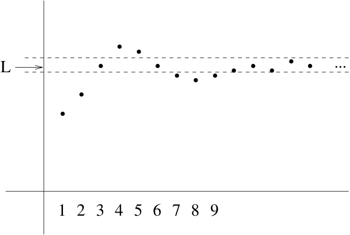
Pictorially, if a sequence has a limit \(L \text{,}\) then for every pair of parallel horizontal lines, however narrow, enclosing the height \(L \text{,}\) the sequence must eventually stay between them. This is shown in Figure 2.21.
As you will see, Proposition 2.28 and Proposition 2.29 give ways to determine limits of more complicated functions once you understand limits of some basic functions. Here is another piece of logic that can help do the same thing. We’ll prove it in class.
Let \(a \) be a real number or \(\pm \infty \) and let \(f, g \) and \(h \) be functions satisfying \(f(x) \leq g(x) \leq h(x) \) for every \(x \text{.}\) If \(\displaystyle\lim_{x \to a} f(x) = L \) and \(\displaystyle\lim_{x \to a} h(x) = L \) then also \(\displaystyle\lim_{x \to a} g(x) = L \text{.}\)
If we know only that \(f(x)\leq g(x)\leq h(x)\) for all \(x\gt a\) and \(\displaystyle\lim_{x \to a^+} h(x)
= \lim_{x \to a^+} h(x) = L \) then we can conclude \(\displaystyle\lim_{x \to a^+}
g(X) = L \text{,}\) and the same for limits from the left.
The same fact is true of sequences: if \(a_n \leq b_n \leq c_n\) for these three sequences and the first and last sequence converge to the same limit \(L \text{,}\) then so does the middle one. We will not do anything with this now, but will get back to this fact in a week or two. The next exercise brushes up on the logical syntax of limits.