Compute the tangent line approximation for \(f(x) := \sqrt[3]{1+x}\) near \(x=0\text{.}\) What quick estimate does this give of \(\sqrt[3]{1.06}\text{?}\) Please check this against a numerical computation on your computer and say how close the quick estimate was.
Unit 5.4 Tangent line estimates and bounds using calculus
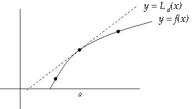
Let’s sum up what we already know about the tangent line approximation, this time in the language of calculus. If \(f\) is a function differentiable in an open interval \(I\) containing \(a\text{,}\) then the tangent approximation to \(f(x)\) at \(a\) is the function
\begin{equation*}
L(x) := f(a) + (x-a) f'(a) \, .
\end{equation*}
Checkpoint 95.
If \(f\) is twice differentiable in \(I\) and \(f'' \geq 0\) on \(I\) then \(L(x) \leq f(x)\) for all \(x \in I\text{,}\) that is, the tangent line approximation is a lower bound for the actual value. Reversing the inequality to \(f'' \leq 0\) reverses the conclusion to \(L(x) \geq f(x)\text{.}\) Making the inequality strict makes the conclusion strict, except at \(a\) where \(f\) and \(L\) always agree; see Figure 5.6.
Checkpoint 96.
Compute the tangent line approximation to \(\sin (\pi/5)\) at any nearby point \(a\) where you know the value of \(\sin (a)\text{.}\) Write the result as an algebraic expression involving \(\pi\) and say whether this is an upper bound, lower bound or neither.
We have said before that \(f(x) \approx L(x)\) when \(x\) is near \(a\text{.}\) How close are these two? At the end of the course you will see that \(L\) is just the first in a series of estimates \(P_1, P_2, \cdots\) that approximate \(f\) better and better. These are the Taylor polynomials, the first being linear, the second quadratic, and so on, the \(n^{th}\) one having degree \(n\text{.}\) Each one is the best approximation for a polynomial of its degree. How good an approximation are they? The degree \(n\) Taylor polynomial differs from \(f\) at \(x\) by a term on the order of \((x-a)^{n+1}\text{.}\) Because the tangent line approximation \(L = P_1\) is the first, it differs from \(f\) by a term on the order of \((x-a)^2\text{,}\) meaning possibly \(2 (x-a)^2\) or \(10 (x-a)^2\) but not anything much bigger than \((x-a)^2\) as \(x \to a\text{.}\)
When talking about orders of magnitude of functions near \(a\text{,}\) recall that higher powers are smaller; that is, \((x-a)^{n+1}\) is smaller than \((x-a)^n\text{.}\) In particular, \((x-a)^2\) is much smaller than \(|x-a|\text{.}\)
The above facts about Taylor polynomials are a preview. We won’t discuss them more now, but instead will focus only on \(P_1\text{,}\) which is also denoted \(L\text{.}\) This proposition is weaker than what we just told you about how close the tangent line approximation is, but has the virtue of being easy to prove.
Proposition 5.7.
The tangent line approximation is better than linear, meaning that
\begin{equation*}
|L(x) - f(x)| \ll |x-a| \qquad \mbox{ as } \qquad x \to a \, ,
\end{equation*}
that is,
\begin{equation*}
\lim_{x \to a} \left | \frac{L(x) - f(x)}{x-a} \right | = 0 \, .
\end{equation*}
Proof.
We need to check that
\begin{equation*}
\lim_{x \to a} \left | \frac{L(x) - f(x)}{x-a} \right | = 0 \, .
\end{equation*}
This follows from
\begin{equation*}
\lim_{x \to a} \frac{L(x) - f(x)}{x-a} = 0
\end{equation*}
by composition with the absolute value function, which is continuous. We evaluate this:
\begin{gather*}
\lim_{x \to a} \frac{f(x) - L(x)}{x-a} = \lim_{x \to a} \frac{f(x) - f(a) - (x-a) f'(a)}{x-a}\\
= \lim_{x \to a} \frac{f(x) - f(a)}{x-a}
+
\lim_{x \to a} \frac{(x-a) f'(a)}{x-a}\\
=f' (a) - f'(a) = 0 \, .
\end{gather*}
Checkpoint 97.
Using a calculator, compute the difference between the cube root of \(1.06\) and your tangent line estimate in Exercise \ref{ex:cube root}. Does this corroborate Proposition \ref{pr:little-o}? Does it corroborate the assertion that \(|P_1 - f|\) should be on the scale of \(|x-a|^2\text{?}\) In each case say why or why not.
Subsection 5.4.1 The mean value theorem
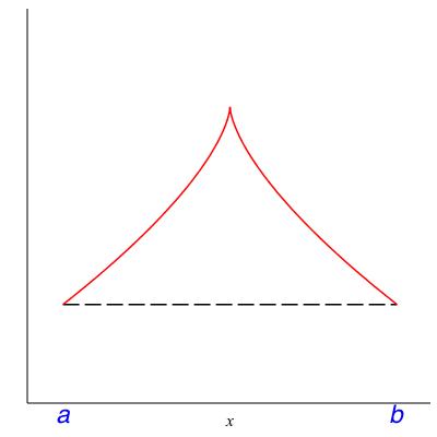
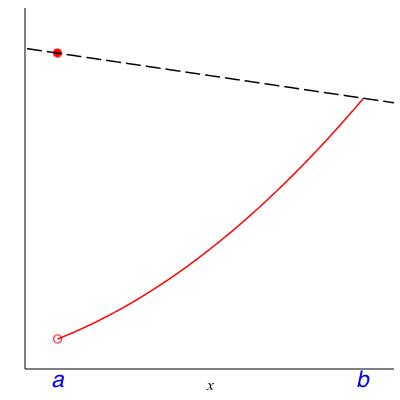
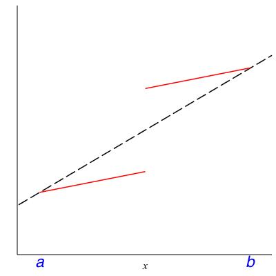
In class we will discuss the following theorem. Please read it now to see whether it makes intuitive sense to you. The hypotheses will be filled in after the class discussion centered on the counterexamples in Figure 5.8.
Theorem 5.9. Mean value theorem.
Let \(f\) be a function and \(a < b\) be real numbers. Assuming some hypotheses, there must be a number \(c \in (a,b)\) where the slope of \(f\) is equal to the average slope over \((a,b)\text{,}\) that is,
\begin{equation}
f'(c) = \frac{f(b) - f(a)}{b-a} \, .\tag{5.2}
\end{equation}
Checkpoint 98.
Let \(f(x)\) be the position (mile marker) of a PA Turnpike driver at time \(x\text{.}\) Suppose the driver entered the Turnpike at Mile 75 (New Stanton) at 4pm and exited at Mile 328 (Valley Forge) at 7pm. What does the Mean Value Theorem tell you in this case? The average slope of \(f\) over interval [4pm,7pm] is the difference quotient \((f(7) - f(4))/(7-4)
= (325 - 75) / 3 = 84 \frac{1}{3}\text{.}\) Thus there is some time \(c\) between 4pm and 7pm that \(f'(c) = 84 \frac{1}{3}\) MPH, in other words, that this driver was traveling at a speed of \(84 \frac{1}{3}\) MPH. Bonus question: can the Mean Value Theorem be used in court by Law Enforcement? It has been ruled in some states that this is legal evidence of the car having violated a speed limit, but not that the particular driver has done so.
Checkpoint 99.
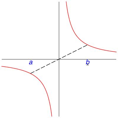
Let \(f(x) := 1/x\) and let \(a < b\) be positive real numbers. What, explicitly in terms of \(a\) and \(b\text{,}\) is the number \(c\) guaranteed by the Mean value theorem?
