Unit 8.2 Optimization in economics and business
Let’s think about production. A standard model, called the Cobb-Douglas production function, says that the productivity of a firm is proportional to both a power of the labor inputs \(L\) and a power of the capital inputs \(K\text{;}\) and that the powers add to 1. That is,
\begin{equation*}
P=kK^\alpha L^\beta
\end{equation*}
where k is the constant of proportionality and \(\alpha+\beta=1\text{.}\) We may as well write \(\beta=1-\alpha\text{,}\) so that our formula reads
\begin{equation*}
P=kK^\alpha L^{1-\alpha}\ .
\end{equation*}
Clearly, if we could increase \(K\) and \(L\) without constraint, we could increase the firm’s output arbitrarily. But we have to operate subject to a budget. Spending more on labor means we have less to spend on capital, and vice versa. We model this by
\begin{equation*}
B=K+L
\end{equation*}
that is, the total budget is the sum of the capital costs and the labor costs.
A natural question to ask is: given a budget, how do we maximize output?
Just as with the window example, we manipulate our constraint to express one variable in terms of the other: \(L=B-K\text{.}\) Then we substitute this into the objective function:
\begin{equation*}
P(K,L(K))=k K^\alpha (B-K)^{1-\alpha}\ .
\end{equation*}
That’s a function we can optimize, on the interval \([0,B]\text{.}\)
Checkpoint 125.
Checkpoint 126.
Now solve symbolically.
If \(\alpha=\frac{1}{3}\text{,}\) express the optimal capital investment in terms of the total budget \(B\text{.}\)
If \(\alpha=\frac{1}{n}\text{,}\) express the optimal capital investment in terms of \(n\) and the total budget \(B\text{.}\)
maximizing profit.
Consider the problem of a firm producing and selling a single good (say, pairs of sneakers). The goal of the firm is to make the most money possible.
Before we get into a precise model, let’s set the ground rules.
- production level
- We’ll call the number of pairs of sneakers we produce \(t\text{.}\)
- production costs
- We’ll write \(C(t)\) for the total cost of producing \(t\) pairs of sneakers. \(C(t)\) is an increasing function.
- markets clear
- We’ll assume that we sell every pair of sneakers we make.
- revenue
- We’ll write \(R(t)\) for the total revenue that selling \(t\) pairs of sneakers brings in. \(R(t)\) is also an increasing function.
- profit
In finance and economics, the adjective marginal is used to denote a derivative. So we say marginal revenue to mean \(R'(t)\) and marginal costs to mean \(C'(t)\text{.}\)
Checkpoint 127.
Based on the assumptions stated above, marginal revenue is
-
sometimes positive
-
sometimes negative
-
always positive
-
always negative
and marginal costs are
-
sometimes positive
-
sometimes negative
-
always positive
-
always negative
.
This use of the word \(marginal\) comes from the fact that, using the tangent line approximation to \(C(t)\text{,}\)
\begin{align*}
C(t+1)&\sim C(t)+C'(t)\left((t+1)-t\right)\\
C(t+1)&\sim C(t)+C'(t)
\end{align*}
In other words, \(C'(t)\) is approximately the additional cost added by the additional pair of sneakers that took us from production level \(t\) to production level \(t+1\text{.}\)
In fact, thinking about derivatives this way can be very useful to understanding the situation of maximizing profit.
Checkpoint 128.
Put yourself in the shoes of a firm manager who gets to decide production levels.
If marginal costs (i.e. cost of producing the next pair of sneakers) are greater than marginal revenues (i.e. revenue generated by the next pair of sneakers), we should
-
increase
-
decrease
-
maintain current level of
the production level.
If marginal costs (i.e. cost of producing the next pair of sneakers) are less than marginal revenues (i.e. revenue generated by the next pair of sneakers), we should
-
increase
-
decrease
-
maintain current level of
the production level.
Be prepared to explain your answer in business terms.
Formally, we’re trying to optimize
\begin{equation*}
P(t)=R(t)-C(t)
\end{equation*}
so our first step ought to be differentiating:
\begin{equation*}
P'(t)=R'(t)-C'(t)\ .
\end{equation*}
We want to find critical points of \(P\text{;}\) that is, we need to solve
\begin{align*}
P'(t)&=0\\
R'(t)-C'(t)&=0\\
R'(t)&=C'(t)
\end{align*}
That is, we’re looking for the production level where marginal cost and marginal revenue are equal.
Checkpoint 129.
As the manager of the firm, it’s your job to occasionally explain your decisions to the firm’s owner (who is mathematically illiterate). The owner sees the phrase marginal profit is zero in your written report and becomes quite upset. “Zero profit?!” he screams.
Explain to the owner why seeking zero marginal profit is the correct business decision.
modeling revenue.
Because profit is the difference of revenue and costs, understand how to solve \(P'(t)=0\) amounts to understanding the revenue function \(R(t)\) and the cost function \(C(t)\text{.}\)
Revenue seems straightforward. If we produce and sell \(t\) pairs of sneakers for a price of \(p\) dollars per sneaker, then
\begin{equation*}
R(t)=p\cdot t
\end{equation*}
But! the more sneakers we produce and sell, the less unique an individual wearing those sneakers is. The more sneakers we produce and sell, the fewer people go unshod. That tends to drive the price down. So the price \(p\) isn’t a constant; it’s a function \(p(t)\) of the number of pairs of sneakers we’ve sold.
Let’s say that we’ve done some market research, and we’ve found that the market price of a pair of sneakers seems to obey
\begin{equation*}
p(t)=300-.05t\text{.}
\end{equation*}
Checkpoint 130.
In the formula \(p(t)=300-.05t\text{,}\) what are the units of each of the following?
-
300:
-
pairs of sneakers
-
dollars
-
pairs of sneaker per dollar
-
dollars per pair of sneakers
-
something else
-
-
t:
-
pairs of sneakers
-
dollars
-
pairs of sneaker per dollar
-
dollars per pair of sneakers
-
something else
-
-
.05:
-
pairs of sneakers
-
dollars
-
pairs of sneaker per dollar
-
dollars per pair of sneakers
-
something else
-
If you said “something else”, find the units.
Interpret what each of these numbers means in terms of the market price for sneakers.
Notice that our model predicts that for high enough levels of production, \(p(t)\) is negative. That is, if we completely saturate the market, we’d have to start paying people to take our sneakers (instead of them paying us). Is this prediction reasonable?
Checkpoint 131.
modeling costs.
What about costs? A standard model of costs is linear:
\begin{equation*}
C(t)=C_0+mt
\end{equation*}
where \(C_0\) is called the fixed cost and represents the costs we have to spend no matter what: capital outlay for the factory, bribes for local politicians, etc.; and \(m\) is the marginal cost (materials and labor to produce a single pair of sneakers).
Checkpoint 132.
Let’s say we build a factory for $10,000 and our marginal cost is $2 per pair of sneakers. Then we have
\begin{equation*}
C(t)=10000+2t
\end{equation*}
and
\begin{equation*}
P(t)=t\cdot(300-.05t)-(10000+2t)\ \ .
\end{equation*}
How do we achieve the maximum profit? When
\begin{equation*}
0=P'(t)=302-.1t
\end{equation*}
which is \(t=3020\text{.}\) The profit we actually make at that production level is \(P(3020)=446,020\text{.}\) Not too bad.
Checkpoint 133.
But costs are not always linear. We say that a cost function obeys economies of scale if the marginal cost gets smaller as we increase the production level. For example, a worker producing their first pair of sneakers might take a lot of time, but by the time they get to their 30\(^{th}\) pair of sneakers, the same worker can probably do so much more quickly (which means the labor cost for that pair of sneakers will be lower.)
Checkpoint 134.
How do we encode economies of scale -- that is, decreasing marginal cost -- in calculus terms?
Just as we did with revenue, we can bootstrap our linear model for costs \(C(t)=C_0+mt\) into a more model by replacing \(m\) with \(m(t)\text{.}\) If we think of our workers in the sneaker factory as gaining skill over time, then we could write something like
\begin{equation*}
m(t)=1+\left(\frac{1}{2}\right)^{t/10}
\end{equation*}
which is to say: the marginal cost starts at $2 per pair of sneakers, has a long-run limit of $1 per pair of sneakers, and every 10 pairs of sneakers produced moves the marginal cost halfway to the long-run limit.
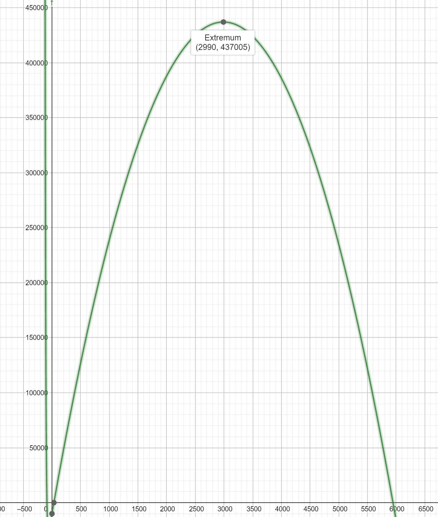
How do we achieve the maximum profit in this case? We have
\begin{align*}
P(t)&=R(t)-C(t)\\
&=t\cdot(300-.05t)-\left(10000+\left(1+\left(\frac{1}{2}\right)^{t/10}\right)t\right)
\end{align*}
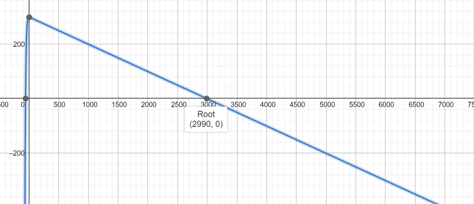
which means that we need to solve
\begin{equation*}
0=P'(t)=299-.1t-\left(\frac{1}{2}\right)^{t/10}-\frac{1}{10}t\ln\left(\frac{1}{2}\right)\left(\frac{1}{2}\right)^{t/10}\ \ .
\end{equation*}
Unfortunately there’s not an algebraically clean solution to this equation, but a graphing utility says that \(t=2990\) is very close.