Several important quantities associated with a probability distribution are the mean, the variance, the standard deviation and the median. We call these summary statistics because they tell us about the probability density as a whole. Again, a couple of paragraphs don’t do justice to these ideas, but we hope they explain the concepts at least a little and make the math seem more motivated and relevant.
Probably the intuitively-simplest summary statistic is the median. This is the \(50^{th}\) percentile of the distribution -- the value of the measured variable which splits the distribution into two equal pieces.
Let’s say our distribution \(X\) represents a length: we pick a board at random from a stack at the hardware store and measure its length in feet. What are the units of:
Each of these definitions looks like the corresponding formula from discrete probability. By way of example, consider the formula for expectation. You might recall what happens when rolling a die. Each of the six numbers comes up about \(1/6\) of the time, so in a large number \(N\) of dice rolls you will get (approximately) \(N/6\) of each of the six outcomes. The average will therefore be (approximately)
When instead there are infinitely many possible outcomes spread over an interval, the sum is replaced by an integral
\begin{equation}
\int_{-\infty}^\infty x \cdot f(x) \, dx \, .\tag{13.3}
\end{equation}
A famous theorem in probability theory, called the Strong Law of Large Numbers, says that the formula (13.3) still computes the long term average: the long term average of independent draws from a distribution with probability density function \(f\) will converge to \(\int x \cdot f(x) \, dx\text{.}\)
The random variable \(X\) has probability density \(2x\) on \([0,1]\text{.}\) If you sample 94 times and take the average of the samples, roughly what will you get?
It is more difficult to understand why the variance has the precise definition it does, but it is easy to see that the formula produces bigger values when the random variable \(X\) tends to be farther from its mean value \(\mu\text{.}\) The standard deviation is another measure of dispersion. To see why it might be more physically relevant, consider the units.
Probabilities such as \(\mathbb{P} (X \in [a,b])\) can be considered to be unitless because they represent ratios of like things: frequency of occurrences within the interval \([a,b]\) divided by frequency of all occurrences. Probability densities, integrated against the variable \(x\) (which may have units of length, time, etc.) give probabilities. Therefore, probability densities have units of "probability per unit \(x\)-value", or in other words, inverse units to the independent variable.
The units of the mean are units of \(\int x f(x) \, dx\text{,}\) which is units of \(f\) times \(x^2\text{;}\) but \(f\) has units of inverse \(x\text{,}\) so the mean has units of \(x\text{.}\) This makes sense because the mean represents a point on the \(x\)-axis. Similarly, the variance has units of \(x^2\text{.}\) It is hard to see what the variance represents physically. The standard deviation, however, has units of \(x\text{.}\) Therefore, it is a measure of dispersion having the same units as the mean. It represents a distance on the \(x\)-axis which is some kind of average discrepancy from the mean.
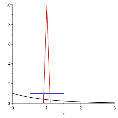
Figure 13.6 shows three probability densities with mean 1. Rank them in order from least to greatest standard deviation. You don’t have to compute precisely unless you want to; just state an answer and justify it intuitively. The three densities are graphed below.