Taylor and Maclaurin polynomials in graphing

Unit 14.2 Taylor and Maclaurin polynomials in graphing

We claimed that the Taylor polynomials are polynomials that "act like" the function \(f(x)\) near \(x=c\text{.}\) What does that mean in terms of the graph of \(f(x)\) and its Taylor polynomials?

🔗

Figure 14.6. Use the checkboxes to display the degrees 1, 2, 3, and 4 Taylor approximations to \(f(x)\text{.}\) You can enter your favorite function \(f(x)\text{,}\) and drag the point \(x=c\) around. Zoom in and out to see how good the approximation is at different scales.

🔗

The fact that the graphs of the Taylor polynomials are similar to those of the original function \(f\) gives us a way to explain why the techniques mentioned in Unit 3.3 work. Let’s imagine the situation of a function \(f(x)\) with \(f(1)=1\text{,}\) \(f'(1)=-\frac{1}{2}\text{,}\) and \(f''(1)=3\text{.}\) This is enough information to compute that the degree-2 Taylor polynomial at \(x=1\) is

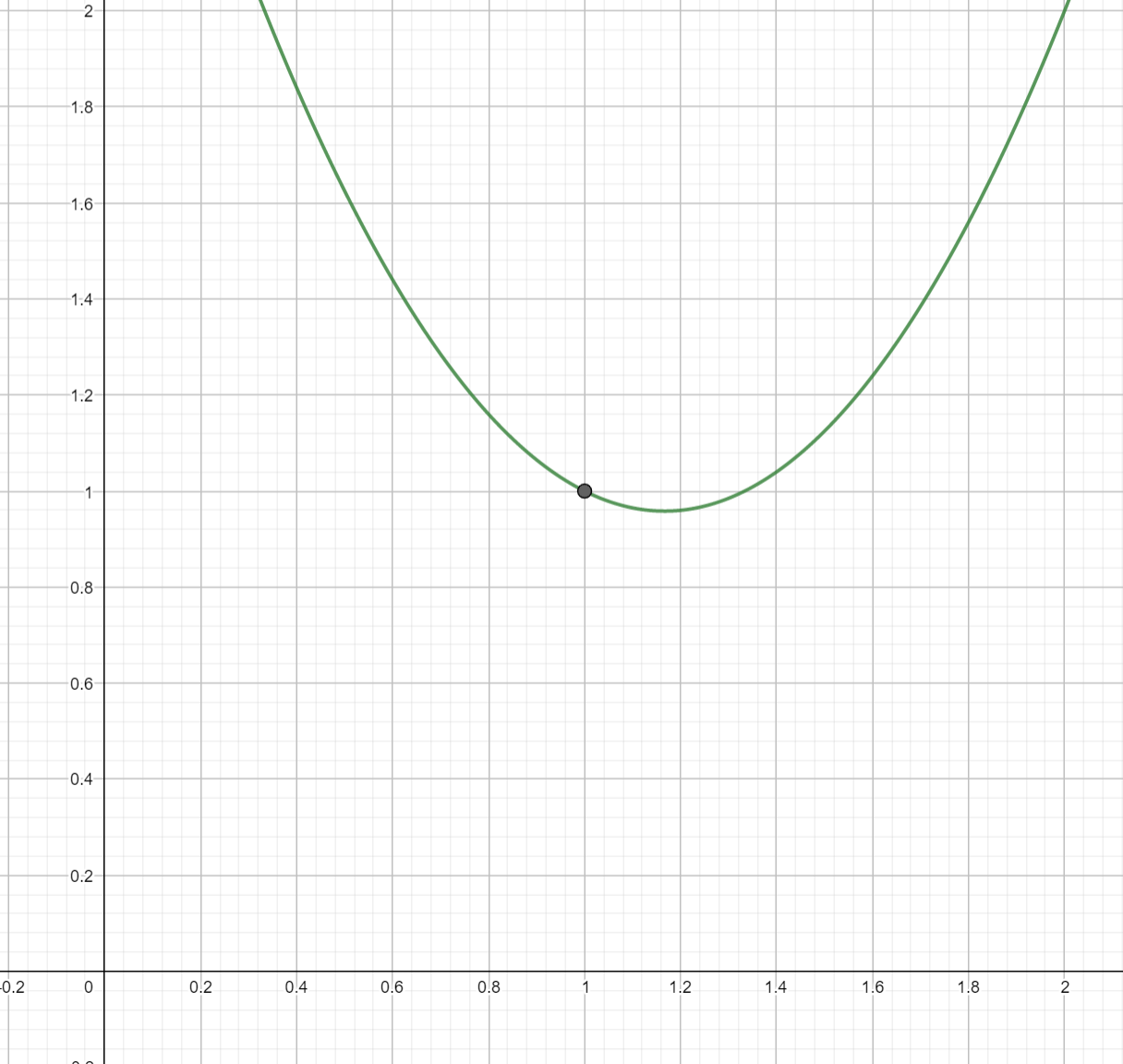
\begin{equation*} P_2(x)=1-\frac{1}{2}(x-1)+\frac{3}{2}(x-1)^2\ \ \ . \end{equation*}

Since the graph of \(P_2\) is close to the graph of \(f\text{,}\) we can infer properties of \(f\) from those of \(P_2\text{.}\)

🔗

Figure 14.7. Even if we only know that \(f(1)=1\text{,}\) \(f'(1)=-\frac{1}{2}\text{,}\) and \(f''(1)=3\text{,}\) we can plot the degree-2 Taylor approximation to \(f\) and learn about how \(f\) behaves near \(x=1\) (indicated by the gray point).
🔗

In particular, we know that any quadratic with a positive coefficient of \(x^2\) has a graph which is an upward-facing parabola. We conclude that \(f\) is concave-up near \(x=1\text{.}\)

🔗

This idea also tells us how to graphically interpret higher derivatives: a function with \(f'''(c)>0\) acts like a cubic with positive leading coefficient; one with \(f^{(4)}(c)\lt 0\) acts like a quartic with a negative leading coefficient; etc.

🔗

Example 14.8.

We want to hand-draw a precise graph of the cosine function near \(x=0\text{.}\)

🔗

The first approach might be to compute some values of cosine near \(x=0\text{,}\) say \(\cos(-.1)\text{,}\) \(\cos(-.2)\text{,}\) \(\cos(.1)\text{,}\) etc. But those are hard to do by hand! So instead, we’ll use a function we know how to compute the values of by hand: the Maclaurin polynomial of degree 2. That’s

\begin{equation*} P_2(x)=1-\frac{1}{2}x^2\ \ \ . \end{equation*}

The values of \(P_2\) are pretty straightforward to compute:

Table 14.9.

🔗

\(x\)	\(P_2(x)\)
\(-.6\)	\(1-\frac{1}{2}(-.6)^2=.82\)
\(-.4\)	\(1-\frac{1}{2}(-.4)^2=.92\)
\(-.2\)	\(1-\frac{1}{2}(-.2)^2=.98\)
\(0\)	\(1\)
\(.2\)	\(1-\frac{1}{2}(.2)^2=.98\)
\(.4\)	\(1-\frac{1}{2}(.4)^2=.92\)
\(.6\)	\(1-\frac{1}{2}(.6)^2=.82\)

and that gives us a decent start to plotting.

🔗

Checkpoint 195.

In the example above, we used the degree-2 Maclaurin polynomial for \(f(x)=\cos(x)\text{.}\) Compute the degree-6 Maclaurin polynomial for \(f(x)=\cos(x)\text{.}\)

🔗

Answer.

\(1-0.5x^{2}+0.0416667x^{4}-0.00138889x^{6}\)

🔗

Prev Top Next