Finding extrema is part of a subject called optimization. The idea is that you control a parameter \(x\) and would like to maximize some objective function \(f(x)\text{,}\) which is perhaps how large you can build something, or perhaps revenue minus cost, or the efficiency of extraction of a natural resource.
The logistic equation models growth rate per unit time, call it \(R\text{,}\) of a population as \(R(x) = C x (A-x)\text{.}\) Here \(C\) is a constant of proportionality, \(x\) is the present population, and \(A\) is a theoretical limit on the population size supported by the habitat. At what size is the population growing the fastest?
We need to find the maximum of \(R(x) := C x (A-x)\) on \([0,A]\text{.}\) The reason for restricting to this interval is that we are told the population size is constrained to be at most \(A\text{,}\) and of course it has to be nonnegative. Computing \(R'(x) = C (A - 2x)\text{,}\) we find \(R' = 0\) for a single value, \(x = A/2\text{.}\) Checking the endpoints, we find \(R\) is zero at both. Therefore the maximum value occurs at \(x = A/2\text{.}\)
Suppose the cost of supplying a station is proportional to the distance from the station to the nearest port, and the cost of the land for the station is inversely proportional to the distance to the nearest port. Adding together these costs, what is the least expensive distance at which to put the station?
Letting \(x\) be the distance to the nearest port and \(f(x)\) be the cost, we are told that \(f(x) = a x + b/x\) where \(a\) and \(b\) are unspecified positive constants. The value of \(f(x)\) is defined for every positive \(x\) and \(f\) is continuous on \((0,\infty)\text{.}\) We seek the global minimum of \(f\) on \((0,\infty)\text{.}\) We are not guaranteed there is a minimum. When we solve for \(f'(x) = 0\) we find
\begin{equation*}
0 = f'(x) = a - \frac{b}{x^2} \, \qquad \mbox{hence} \qquad x
= \sqrt{\frac{b}{a}} \, .
\end{equation*}
At this value, \(f(x) = a \sqrt{\frac{b}{a}} + b/\sqrt{\frac{b}{a}}
= 2 \sqrt{ab}\text{.}\) Checking what happens near 0 and \(\infty\text{,}\) we find \(\displaystyle\lim_{x \to 0} f(x) = \infty\) and \(\displaystyle\lim_{x \to \infty} f(x) = \infty\text{.}\) Therefore, there is a minimum value, which we have determined to be \(\sqrt{ab}\) occuring at \(x = \sqrt{\frac{a}{b}}\text{.}\)
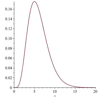
The functions \(x^\gamma e^{-x}\text{,}\) for \(x \geq 0\text{,}\) arise in probability modeling. They are called Gamma densities. We will return to these in Chapter 13. For now, we would like to understand the shape of these functions. An example with \(m=5\) is shown in Figure 7.23.
The place where one is most likely to find the random variable is where the maximum of the density occurs. Where does the maximum of \(f(x) := x^5 e^{-x}\) occur? We know that the value is zero at \(x=0\) and positive everywhere else. We also know \(\displaystyle\lim_{x \to \infty} f(x) = 0\text{.}\) This means there must be a maximum at some positive finite \(x\text{.}\) The function \(f\) is differentiable for all positive \(x\text{,}\) therefore the maximum can only occur where \(f' = 0\text{.}\) Solving
Let \(h\) be the height of a member of a carnivore species. In this simple model, the food gathering capability of an individual is given by \(k h^2\) while its daily food needs are given by \(c h^3\text{.}\)
We can only make educated guesses about the reason the equations in the model have this form. If an animal’s speed is proportional to its height then the model stipulates territory is proportional to the square of this. Perhaps territory is the area that can be reached in a given amount of time such as an hour or a day. As to why food needs would be proportional to volume, one might imagine that sustaining and nourishing tissue requires nutrients proportional to volume.
Units of \(c\) are food per length\(^3\) and units of \(k\) are food per length\(^2\text{.}\) For example, if food is measured in kilograms and length in meters, then food per length\(^3\) would be kg/m\(^3\text{;}\) however one might measure food in other ways such as calories, or numbers of a particular animal of prey, etc.
To maximize food gathering ability minus food needs, how tall should members of this species be?
The objective function we want to maximize is \(k h^2 - c h^3\text{.}\) Having been told no limitations on size, we assume \(h\) can be any positive real number, though we may have to retract that if the optimum turns out to have unrealistic scale. Differentiating \(f(h) := k h^2 - c h^3\) with respect to \(h\) yields \(2 k h - 3 c h^2\) and setting equal to zero gives the two solutions \(0\) and \(x_* := (2k) / (3c)\text{.}\) This indeed has units of length. Clearly \(f(0) = 0\text{.}\) The value of the objective function at \(x_*\) is \(4 k^3 / (27 c^2)\text{,}\) which is positive. Therefore the maximum of \(f\) on \([0,\infty)\) is either \(4 k^3 / (27 c^2)\) achieved at \(h = (2k) / (3c)\) or there is no maximum because the function can get arbitrarily large as \(h \to \infty\text{.}\) At infinity, \(f(h) \sim - c h^3\) because \(k h^2 \ll c h^3\) as \(h \to \infty\text{.}\) Therefore, \(h\) has a maximum at a positive location, whose value is \(4 k^3 / (27 c^2)\)
Continuing the previous example, suppose that for lions \(k = 0.001\) gazelles per square meter, and \(c = 0.0004\) gazelles per cubic meter. What length of lion maximizes its excess food gathering ability, and how many gazelle carcasses per day will be left over for the other lions in the pride?