Unit 10.2 Riemann sums and the definite integral
With this build up, we will give a mathematical definition for the area for a certain restricted class of shapes. These are rectangular on three sides but whose top is described by a continuous function. More precisely, let \(a \lt b\) be real numbers and let \(f\) be positive and continuous on the closed interval \([a,b]\text{.}\) We will define the area of the region \(R\) bounded on the left by the vertical line \(x=a\text{,}\) on the right by the vertical line \(x=b\text{,}\) on the bottom by the \(x\)-axis (the line \(y=0\)), and on the top by the graph of \(f\) (the curve \(y = f(x)\)). This region is shown in Figure 10.3.
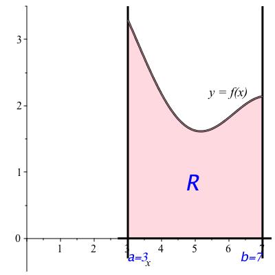
region between the \(x\)-axis and the graph of a function
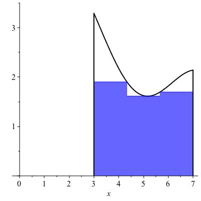
We now define the lower and upper Riemann sums with \(n\) rectangles for a function \(f\) on an interval \([a,b]\text{.}\) If you prefer a picture, refer to Figure 10.4.

Checkpoint 150.
Definition 10.5.
Let \(f\) be a nonnegative continuous function on an interval \([a,b]\) and let \(n\) be a positive integer. Let \(I_1, \ldots , I_n\) denote the intervals you get when you divide \([a,b]\) into \(n\) equally sized intervals. For each interval \(I_k\text{,}\) let \(y_k\) be the minimum value of \(f\) on \(I_k\) and let \(R_k\) be the rectangle with base \(I_k\) on the \(x\)-axis and height \(y_k\text{.}\) The lower Riemann sum for \(f\) on \([a,b]\) with \(n\) rectangles is the sum of the areas of the rectangles \(R_k\text{,}\) for \(1 \leq k \leq n\text{.}\) The upper Riemman sum is defined similarly, with the maximum value instead of the minimum value on each interval.
Checkpoint 151.
Example 10.6.
We are not given precise values for the function \(f\) in Figure 10.4, but we can estimate from the graph. The rectangles each have width \(4/3\text{.}\) The respective heights for the lower Riemann sum appear to be roughly \(1.9, 1.6\) and \(1.7\text{,}\) making the lower Riemann sum equal to \((4/3) 1.9 + (4/3) 1.6 + (4/3) 1.7
= (4/3) 5.2 \approx 6.93\text{.}\) The upper Rieman sum is computed from rectangles with approximate heights \(3.3, 1.9\) and \(2.15\text{,}\) leading to a total area of \((4/3) 7.35 = 9.8\text{.}\)
left and right Riemann sums
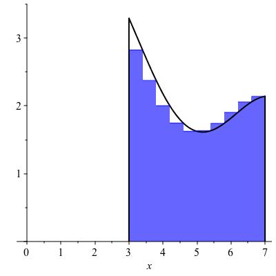
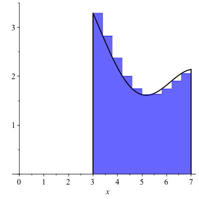
The left Riemann sums and right Riemann sums are defined similarly, except that instead of using the minimum or maximum values of the function on each sub-interval the left Riemann sums uses the value at the left endpoint of each interval \(I_k\text{,}\) while the right Riemann sum uses the value at the right endpoint of each sub-interval \(I_k\text{.}\) Examples are shown in Figure 10.7.
Checkpoint 152.
The upper and lower Riemann sums give upper and lower bounds on the area of the figure. The left and right Riemann sums are neither upper nor lower bounds for the area, but they are sandwiched in between the lower and upper Riemann sums, so they also converge to the area. They are useful because always choosing the left endpoint (or always choosing the right endpoint) leads to a simpler formula.
Checkpoint 153.
Write a summation formula for the left Riemann sum for \(f\) on \([a,b]\) with 10 rectangles. It should have 10 terms and look like this:
\(\displaystyle\sum_{n=1}^{10}\)
The values of the lower and upper Riemann sums in Figure 10.4 are approximately \(6.9\) and \(9.8\text{.}\) These are not very close to each other, leaving considerable uncertainty about the true area. Replacing by the left (say) Riemann sums, we can program the sum into a computing device and compute for much greater values of \(n\text{.}\) If we increase \(n\) from 3 to 10, as in Figure 10.7, we find the Riemann sums come out to approximately 8.48 and 8.02 -- somewhat better. These are not necessarily bounds: the true value could be greater than both, or less than both, or in between. Replacing \(n\) by 50 gives 8.28. This is again not a bound, however the following theorem guarantees that as \(n \to \infty\text{,}\) this will converge to the area.
Theorem 10.8.
The upper Riemann sums for any continuous function \(f\) on any closed interval \([a,b]\) converge as \(n \to \infty\text{.}\) The lower Riemann sums converge to the same value. It follows that you can let \(y_k = f(x_k)\) for any \(x_k \in I_k\) and the sums of rectangle areas will still converge to this common limit.
Definition 10.9.
The common limit in Theorem 10.8 is called the definite integral of \(f\) from \(a\) to \(b\) and is denoted \(\displaystyle\int_a^b f(x) \, dx\text{.}\)
Checkpoint 154.
Remark 10.10.
The variable \(x\) is a bound variable; the notation \(\displaystyle\int_a^b f(u) \, du\) would represent the same thing. Also, as in the notation for derivatives, you shouldn’t try to interpret what the symbol \(du\) means on its own. It evokes the width of an infinitesimal rectangle, but you can’t always count on it to behave nicely in equations.
Checkpoint 155.
From this construction and theorem, you can deduce some identities for integrals.
Let’s say we know that \(\displaystyle\int_a^bf(x)\ dx=3\) and \(\displaystyle \int_b^c f(x)\ dx=5\text{.}\) Compute each of the following:
-
\(\displaystyle\int_a^b f(x) \, dx + \displaystyle\int_b^c f(x) \, dx=\)
-
\(\displaystyle\int_a^b 3 + 10 f(x) \, dx=\)
