Area is the most visually obvious interpretation but there are many others. If material (or charge, or mass, etc.) is spread out unevenly over an interval, the density at any point is the amount of material per length near that point. It has units of material divided by length. The total amount of material in the interval is gotten by summing how the amount of material over small intervals. When the interval is small enough, we can estimate the amount of material as \(f(x)\) times the length of the interval where \(x\) is any point in the interval. This is not exact because \(f\) generally will still vary over the interval, but not by much when \(x\) is small. The limit as the interval lengths go to zero will be \(\displaystyle\int_a^b f(x) \, dx\) and will represent the total material.
A 3-inch blade of grass is covered in mold. The amount of mold decreases up the blade because it is killed by sunlight. The density of mold per inch is \(1000 e^{-x/3}\) spores per inch at height \(x\) inches from the ground. The total number of spores on the blade of grass is given by \(\displaystyle\int_0^3 1000 e^{-x/3} \, dx\text{.}\)
Integrals can also be used to give averages. For a finite collection, the average is defined to be the total divided by the number you added to get the total. Averages over an interval are defined similarly.
The average of a quantity varying over an interval \([a,b]\) according to a function \(f\) is defined to be \(\frac{1}{b-a} \displaystyle\int_a^b f(x) \, dx\text{.}\)
Suppose the temperature over a day is \(f(t)\) degrees Celsius \(t\) hours after midnight. The average temperature over the day is then \(\frac{1}{24} {\displaystyle\int_0^{24} f(t) \, dt}\text{.}\)
Suppose \(f(x)\) is some constant \(c\) on the interval \([a,b]\text{.}\) Intuitively, what is the average of \(f\) on \([a,b]\text{?}\) Compute the average value of \(f\) on \([a,b]\) directly from the definitions and check that it is what you expected.
An integral is a limit of a sum of rectangles’ areas. The units are therefore the same units as the rectangles’ areas. The rectangles live on a graph where the \(x\)-axis has units of the argument variable and the \(y\)-axis has units of the function. Therefore the rectangle units, hence the integral units, are units of the argument times units of the function. In the grass example, the function was density (spores per inch) and the argument was inches, therefore the integral had units of spores. It is a good thing that this agrees with our interpretation of the integral as the total number of spores. In the temperature example, \(f\) has units of temperature and \(t\) is in units of time, so the integral of \(f\) has units of temperature times time. This sounds like a strange unit but it’s not unheard of. Severity of cold spells is measured, for example, in heating degree-days. The average is the integral divided by the time, so it is in units of temperature. Of course: the average temperature should be a temperature!
In physics there are countless things represented by integrals. One is the moment. Suppose mass is spread out along \([a,b]\) with density \(f\) (you know what that means now, right?). Integrate \(f\) and you get the total mass. If instead you compute \(\displaystyle\int_a^b x \, f(x) \, dx\) you get the moment of inertia, which tells you how much the weight counts when balancing (imagine a teeter-totter pivoting on the origin), or how much torque is needed to produce a given angular acceleration.
In probability theory, random quantities can be discrete or continuous. If the random quantity \(X\) is discrete it means that there is a sset of values \(x_1, x_2 , \ldots\) such that probabilities for \(X = x_k\) sum to 1. This could be a finite sum or the sum of an infinite sequence (you now know the definition of an infinite sum, right?). For continuous quantities, you need integrals. The probabilities for finding \(X\) to take various values are spread continuously over an interval (possibly an infinite interval such as the whole real line). There will be a probability density function \(f\) such that the probability of finding \(X\) in a given interval \([a,b]\) will be \(\displaystyle\int_a^b f(x) \, dx\text{.}\) We will say more about this in Chapter 12, after we have defined integrals where one or both of the limits of integration can be infinite.
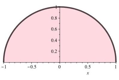
Going back to the area interpretation, you may ask what about more general shapes? It turns out you don’t really need straight sides. The vertical walls on the left and right sides of the regions Figure 10.3 and Figure 10.4 can disappear. For example, letting \(f(x) =
\sqrt{1-x^2}\) and \([a,b] = [-1,1]\) produces the upper half of a disk.
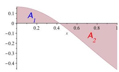
Let \(\Delta_k\) denote the width of \(I_k\text{.}\) The most useful definition turns out to be that the integral is still the limit of sums of the quantities \(\displaystyle\sum_k f(x_k) \cdot \Delta_k\) but we must interpret this as a new concept, called signed area rather than area. We won’t worry too much about signed area; it just means we need to keep track of whether \(f\) is positive or negative before we know whether \(\displaystyle\int_a^b f(x) \, dx\) computes area or its negative. Figure 10.17 shows a function which is positive on \([0,0.42]\) and negative on the interval \([0.42,1]\text{.}\) The integral \(\displaystyle\int_0^1 f(x) \, dx\) will be slightly negative because it adds a positive area \(A_1\) to a negative signed area \(A_2\text{.}\)
Suppose \(f\) and \(g\) are functions such that \(f \geq g\) on \([a,b]\text{.}\) One interpretation of \(\displaystyle\int_a^b [f(x) - g(x)] \, dx\) is that it is the area of the shape with upper boundary \(f\) and lower boundary \(g\text{.}\)
We started out computing areas of a very specific set of shapes, looking like three sides of a rectangle and a possibly curved upper boundary. Using the idea of upper and lower boundaries we can use integrals to give the area of a much greater variety of shapes.
On a coordinate axis, draw a heart shape (you know, the classic Valentine’s heart). Then draw in values \(a\) and \(b\) on the \(x\)-axis and graphs of functions \(f\) and \(g\) such that the area of the heart is computed by \(\displaystyle\int_a^b [f(x) - g(x)] \, dx\text{.}\)
The examples of densities of quantities spread out along a line is somewhat limited. When quantities spread out, usually they spread over a region in a plane or in three dimensions.
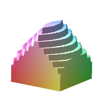
The next course in this sequence covers multivariable integration. Still, there are some higher dimensional things you can do with ordinary integrals. One of these is to compute a volume of an object if you know the area of its cross-sections. Dividing the object into \(n\) very thin slabs, the volume of the \(k^{th}\) one is roughly the thickness \(\Delta_k\) times the cross-sectional area of the \(k^{th}\) slab, call it \(A_k\text{;}\) see Figure 10.19.
The limit of \(\displaystyle\sum_{k=1}^n A_k \Delta_k\) should give the volume. Line up the slabs so that the \(x\)-axis goes perpendicular to the slabs. This limit looks awfully similar to the limit of \(\displaystyle\sum_{k=1}^n f(x_k) \Delta_k\) where \(x_k\) is any point on the \(x\)-axis inside the \(k^{th}\) slab and \(f\) is the function telling the cross-sectional area at every \(x\)-value. Therefore, the volume is computed by \(\displaystyle\int_a^b f(x) \, dx\) where \(a\) and \(b\) are the \(x\)-values at the first and last slab respectively.
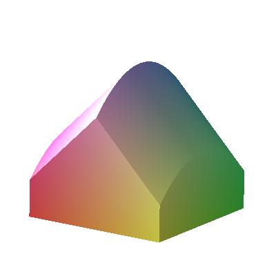
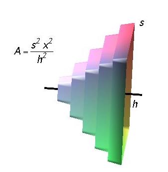
We write an integral for volume of a pyramid whose base is a square of side length \(s\) and whose height is \(h\text{.}\) It corresponds best to the description above if we orient it so the height is measured along the \(x\)-direction with the apex at the origin. See Figure 10.21. The cross-section is a square with side increasing linearly from 0 to \(s\) as \(x\) increases from 0 to \(h\text{.}\) Thus, the side length is given by \(\ell (x) = (s/h) x\text{,}\) hence the cross-sectional area is given by \(f(x) = (s/h)^2 x^2\) between \(x=0\) and \(x=h\text{.}\) The volume is therefore given by \(\displaystyle\int_0^h (s/h)^2 x^2 \, dx\text{.}\) When you learn to compute integrals, this will turn out to be a pretty easy one.