Unit 14 Integration and Probability
Maybe you've taken a courses in probability. Maybe you saw a little probability theory in high school. Maybe you've never studied anything to do with probability.
The first thing students usually learn is discrete probability, where the random variables take values in a finite set, with given probabilities for each outcome. That's because this can be studied with middle school mathematics. For example, rolling two 6-sided dice leads to 36 possible outcomes, each equally likely; this in turn leads to 11 possible outcomes for the sum of the two dice, with probabilities ranging from \(1/36\) for 2 and 12 to \(6/36\) for 7. All questions about rolls of finitely many dice can be answered with careful thinking and basic arithmetic.
Random variables whose values are spread over all real numbers, or a real interval, require calculus even to define (much less to study). These are called continuous random variables, and are the topic of this section.
Philosophically, a real-valued random variable \(X\) is a quantity that has a value equal to some real number, but will have a different value each time some kind of experiment is run. It is unpredictable, therefore we cannot answer the question "What is the value of \(X\text{?}\)" but only "What is the probability that the value of \(X\) lies in the set \(A\text{?}\)"
For example, suppose we throw a dart at a 12 foot wide wall, from a long enough distance and with poor enough aim that it is as likely to hit any region as any other (if we miss completely, we get another try). Say the random variable \(X\) is the distance (in feet) from the left edge of the wall. We can ask for the probability that \(X \leq 2\text{,}\) that is that the dart lands within two feet of the left edge.
Checkpoint 168.
What should this probability be? Forget about calculus, just use your intuition.
\(0.166667\)
Subsection 14.1 Probability densities
For discrete random variables you answer this type of question by summing the probability that \(X\) is equal to \(y\) for every \(y\) in the set \(A\text{.}\) For continuous random variables, the probability of being equal to any one real number is zero. In the example with the dart, the probability that it lands exactly \(\sqrt{3}\) feet from the left edge (or 1 foot, or \(1/3\) of a foot, or any other real number of feet) is zero. The only way to get a nonzero probability is to consider an entire interval of values. Thus the most basic questions we ask about \(X\) are: what is the probability that \(X \in [a,b]\text{,}\) where \(a \lt b\) are fixed real numbers. These probabilities will be governed by a probability density, which is a nonnegative function telling how likely it is for \(X\) to be in an interval centered at any given real number.
Definition 14.1. probabilitiy densities.
- probability density
- A probability density is a nonnegative function \(f\) such that \(\int_{-\infty}^\infty f(x) \, dx = 1\text{.}\)
- random variable
- A random variable \(X\) is said to have probability density \(f\) if the probability of finding \(X\) in any interval \([a,b]\) is equal to \(\int_a^b f(t) \, dt\text{.}\)
- probability
- We denote the probability of finding \(X\) in \([a,b]\) by \(\mathbb{P} (X \in [a,b])\text{.}\)
Checkpoint 169.
Sometimes \(f\) is defined only on an interval \([a,b]\) and not on the whole real line. The interpretation is that the random variable \(X\) takes values only in \([a,b]\text{.}\) Probabilities for \(X\) are then defined by integrating in sub-intervals of \([a,b]\text{.}\) Often one extends the definition of \(f\) to all real numbers by making it zero off of \([a,b]\text{.}\) This may result in \(f\) being discontinuous but its definite integrals are still defined.
Example 14.2.
The standard exponential random variable has density \(e^{-x}\) on \([0,\infty)\text{.}\) If \(X\) has this density, what is \(\mathbb{P} (X \in [-1,1])\text{?}\) This is the same as \(\mathbb{P} (X \in [0,1])\text{,}\) because by assumption \(X\) cannot be negative. We compute it by \(\displaystyle \int_0^1 e^{-x} \, dx = \left. e^{-x} \right |_0^1 = 1 - e^{-1}\text{.}\) As a quick reality check we observe that the quantity \(1 - \frac{1}{e}\) is indeed between zero and one, therefore it makes sense for this to be a probability.
Checkpoint 170.
Write the statement \(X \geq m\) as a statement about \(X\) being in a (possibly infinite) interval. Letting \(f\) be the probability density of \(X\text{,}\) write an integral computing \(P (X \geq m)\text{.}\)
Often the model dictates the form of the function \(f\) but not a multiplicative constant.
Example 14.3.
For example, if we know that \(f(x)\) should be of the form \(C x^{-3}\) on \([1,\infty)\) then we would need to find the right constant \(C\) to make this a probability density. The function \(f\) has to integrate to 1, meaning we have to solve
for \(C\text{.}\) Solving this results in \(C = 2\text{,}\) therefore the density of \(f\) is \(2 / x^3\) on \([1,\infty)\text{.}\)
Checkpoint 171.
Suppose \(X\) has density proportional to \(\cos (x)\) on the interval \([-\pi/2 , \pi / 2]\text{.}\) What value of \(C\) makes \(C \cos x\) a probability density on this interval?
\(0.5\)
Subsection 14.2 Summary statistics
Several important quantities associated with a probability distribution are the mean, the variance, the standard deviation and the median. We call these summary statistics because they tell us about the probability density as a whole. Again, a couple of paragraphs don't do justice to these ideas, but we hope they explain the concepts at least a little and make the math seem more motivated and relevant.
Probably the intuitively-simplest summary statistic is the median. This is the \(50^{th}\) percentile of the distribution -- the value of the measured variable which splits the distribution into two equal pieces.
Definition 14.4.
The median of a random variable \(X\) having probability density \(f\) is the real number \(m\) such thatCheckpoint 172.
Definition 14.5.
- mean
- If \(X\) has probability density \(f\text{,}\) the mean or expectation of \(X\) (the two terms are synonyms) is the quantity\begin{equation} \mathbb{E} X := \int_{-\infty}^\infty x \, f(x) \, dx.\label{eq-expectation}\tag{14.2} \end{equation}A variable commonly used for the mean of a distribution is \(\mu\text{.}\)
- variance
- If \(X\) has probability density \(f\) and mean \(\mu\text{,}\) the variance of \(X\) is the quantity\begin{equation*} \operatorname{Var} (X) := \int_{-\infty}^\infty (x - \mu)^2 \, f(x) \, dx \, . \end{equation*}
- standard deviation
- The standard deviation of \(X\) is just the square root of the variance\begin{equation*} \sigma := \sqrt{\operatorname{Var} (X)} \, . \end{equation*}
Checkpoint 173.
Let’s say our distribution \(X\) represents a length: we pick a board at random from a stack at the hardware store and measure its length in feet. What are the units of:
the median
the mean \(\mu=\mathbb{E}(X)\text{:}\)
the variance \(\operatorname{Var}(X)\text{:}\)
the standard deviation \(\sigma\text{:}\)
Why do you think we take the square root of the variance?
Each of these definitions looks like the corresponding formula from discrete probability. By way of example, consider the formula for expectation. You might recall what happens when rolling a die. Each of the six numbers comes up about \(1/6\) of the time, so in a large number \(N\) of dice rolls you will get (approximately) \(N/6\) of each of the six outcomes. The average will therefore be (approximately)
We can write this in summation notation as
If we think of this sum as a Riemann sum for something, and do our Greek-to-Latin trick, we get back the formula (14.2).
Checkpoint 174.
A carnival game that costs a dollar to play gives you a quarter for each spot on a roll of a die (e.g., 75 cents if you roll a 3).
When you have spent \(N\) dollars, about how much money (in dollars) will you have received? Give a formula involving the variable \(N\text{.}\)
Should you play this game?
yes -- you will tend to make money
no -- you will tend to lose money
who cares? In the long run you'll break even.
When instead there are infinitely many possible outcomes spread over an interval, the sum is replaced by an integral
A famous theorem in probability theory, called the Strong Law of Large Numbers, says that the formula (14.3) still computes the long term average: the long term average of independent draws from a distribution with probability density function \(f\) will converge to \(\int x \cdot f(x) \, dx\text{.}\)
Checkpoint 175.
It is more difficult to understand why the variance has the precise definition it does, but it is easy to see that the formula produces bigger values when the random variable \(X\) tends to be farther from its mean value \(\mu\text{.}\) The standard deviation is another measure of dispersion. To see why it might be more physically relevant, consider the units.
Probabilities such as \(\mathbb{P} (X \in [a,b])\) can be considered to be unitless because they represent ratios of like things: frequency of occurrences within the interval \([a,b]\) divided by frequency of all occurrences. Probability densities, integrated against the variable \(x\) (which may have units of length, time, etc.) give probabilities. Therefore, probability densities have units of "probability per unit \(x\)-value", or in other words, inverse units to the independent variable.
The units of the mean are units of \(\int x f(x) \, dx\text{,}\) which is units of \(f\) times \(x^2\text{;}\) but \(f\) has units of inverse \(x\text{,}\) so the mean has units of \(x\text{.}\) This makes sense because the mean represents a point on the \(x\)-axis. Similarly, the variance has units of \(x^2\text{.}\) It is hard to see what the variance represents physically. The standard deviation, however, has units of \(x\text{.}\) Therefore, it is a measure of dispersion having the same units as the mean. It represents a distance on the \(x\)-axis which is some kind of average discrepancy from the mean.
Checkpoint 176.
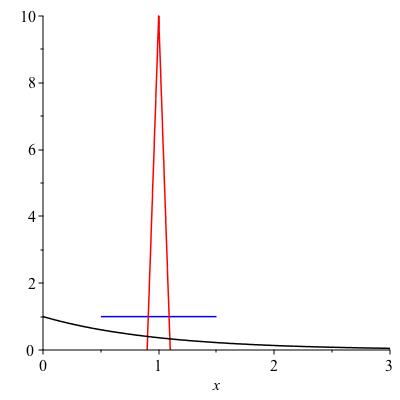
Figure 14.6 shows three probability densities with mean 1. Rank them in order from least to greatest standard deviation. You don’t have to compute precisely unless you want to; just state an answer and justify it intuitively. The three densities are graphed below.
\(f(x) := 1\) on \([1/2,3/2]\) (blue)
\(f(x) := 10 - 100 \lvert x-1\rvert\) on \([0.9,1.1]\) (red)
\(f(x) := e^{-x}\) on \([0,\infty)\) (black)
(least standard deviation)
blue distribution
red distribution
black distribution
blue distribution
red distribution
black distribution
blue distribution
red distribution
black distribution
Subsection 14.3 Some common probability densities
There are a zillion different functions commonly used for probability densities. Three of the most common are named in this section: the exponential, the uniform, and the normal. These are common in probability for reasons analogous to why exponential behavior is common in evolving systems. Each of these is constructed to have a particular useful property.
The uniform distribution, as the name applies, arises when a random quantity is uniformly likely to be anywhere in an interval. It is often used as an "uninformed" model when all you know is that a quantity has to be somewhere in a fixed interval. The normal arises when many small independent contributions are summed. It is often used to model observational error. The exponential is the so-called memoryless distribution. It arises when the probability of finding \(X\) in the next small interval, given that you haven't already found it, is always constant.
All three of these are parametrized families of distributions. Once values are picked for the parameters you get a particular distribution. This section concludes by giving definitions of eac h and discuss typical applications.
The exponential distribution.
The exponential distribution has a parameter \(\mu\) which can be any positive real number. Its density is \((1/\mu) e^{-x/\mu}\) on the positive half-line \([0,\infty)\text{.}\) This is obviously the same as the density \(C e^{-Cx}\) (just take \(C = 1/\mu\)) but we use the parameter \(\mu\) rather than \(C\) because a quick computation shows that \(\mu\) is a more natural property of the distribution.
Checkpoint 177.
The exponential distribution has a very important "memoryless" property. If \(X\) has an exponential density with any parameter and is interpreted as a waiting time, then once you know it didn't happen by a certain time \(t\text{,}\) the amount of further time it will take to happen has the same distribution as \(X\) had originally. It doesn't get any more or any less likely to happen in the the interval \([t,t+1]\) than it was originally to happen in the interval \([0,1]\text{.}\)
The median of the exponential distribution with mean \(\mu\) is also easy to compute. Solving \(\int_0^M \mu^{-1} e^{-x/\mu} \, dx = 1/2\) gives \(M = \mu \cdot \ln 2\text{.}\) When \(X\) is a random waiting time, the interpretation is that it is equally likely to occur before \(\ln 2\) times its mean as after. Because \(\ln 2 \approx 0.7\text{,}\) the median is significantly less than the mean. When modeling with exponentials, it is good to remember it produces values that are unbounded but always positive.
Any of you who have studied radioactive decay know that each atom acts randomly and independently of the others, decaying at a random time with an exponential distribution. The fraction remaining after time \(t\) is the same as the probability that each individual remains undecayed at time \(t\text{,}\) namely \(e^{-t/\mu}\text{,}\) so another interpretation for the median is the half-life: the time at which only half the original substance remains. Other examples are the life span of an organism that faces environmental hazards but does not age, or time for an electronic component to fail (they don't seem to age either).
The uniform distribution.
The uniform distribution on the interval \([a,b]\) is the probability density whose density is a constant on this interval: the constant will be \(1/(b-a)\text{.}\) This is often thought of the least informative distribution if you know that the the quantity must be between the values \(a\) and \(b\text{.}\) The mean and median are both \((a+b)/2\text{.}\)
Checkpoint 178.
Use calculus to prove that a constant function \(C\) on an interval \([a,b]\) is a probability density if and only if \(C = \frac{1}{b-a}\text{.}\)
Example 14.7.
In your orienteering class you are taken to a far away location and spun around blindfolded when you arrive. When the blindfold comes off, you are facing at a random compass angle (usually measured clockwise from due north). It would be reasonable to model this as a uniform random variable from the interval \([0,360]\) in units of degrees.
Checkpoint 179.
The normal distribution.
The normal density with mean \(\mu\) and standard deviation \(\sigma\) is the density
The standard normal is the one with \(\mu = 0\) and \(\sigma = 1\text{.}\) There is a very cool mathematical reason for this formula, which we will not go into. When a random variable is the result of summing a bunch of smaller random variables all acting independently, the result is usually well approximated by a normal. It is possible (though very tricky) to show that the definite integral of this density over the whole real line is in fact 1 (in other words, that we have chosen the right constant to make it a probability density).
Annoyingly, there is no nice antiderivative, so no way in general of computing the probability of finding a normal between specified values \(a\) and \(b\text{.}\) Because the normal is so important in statistical applications, they made up a notation for the indefinite integral in the case \(\mu = 0, \sigma = 1\text{,}\) using the capital Greek letter \(\Phi\) ("phi", pronounced "fee" or "fie"):
So now you can say that the probability of finding a standard normal between \(a\) and \(b\) is exactly \(\Phi (b) - \Phi (a)\text{.}\) In the old, pre-computer days, they published tables of values of \(\Phi\text{.}\) It was reasonably efficient to do this because you can get the antiderivative \(F\) of any other normal from the one for the standard normal by a linear substition: \(F(x) = \Phi \left(\frac{x-\mu}{\sigma}\right)\text{.}\)