Unit 7 Asymptotic analysis and L'Hôpital's Rule
When you learn about complex numbers, they seem in one sense like make-believe but in another sense like ordinary math because they obey clear rules. Learning about infinity is different. The word is in the vocabulary of most children, but no one knows the rules. Is infinity part of math? Part of philsophy? Science fiction? It turns out infinity does obey some very clear rules, as long as you decide to define it as a limit. (Trust mathematicians to take the fun out of it!)
Suppose, in addition to the real numbers, we include the numbers \(+\infty, -\infty\) and UND (for undefined). These are the possible limits a function can have. The goal is to create combining rules for limits under the basic operations: addition, subtraction, multiplication, division and taking powers. One rule is that once something is undefined, it stays that way. Limits that DNE could turn out to be \(\pm \infty\) rather than UND, but once a limit gets classified as UND, nothing can be inferred about what you get when you add it to something, multiply it, etc. Thus, UND + 3, UND \(- \infty\text{,}\) \(-\infty \cdot\) UND and UND / UND are all undefined. For the remaining situations, the definition is as follows.
Definition 7.1.
If \(a, b\) and \(L\) are real numbers or \(\pm \infty\text{,}\) and \(\odot\) is an operation, we say \(a \odot b = L\) if for every \(f\) and \(g\) such that \(\lim_{x \to 0} f(x) = a\) and \(\lim_{x \to 0} g(x) = b\text{,}\) it is always true that \(\lim_{x \to 0} f(x) \odot g(x) = L\text{.}\)
Example 7.2. \(\infty + 3\).
The definition allows us to check if any guess is right. Let's guess \(\infty + 3 = \infty\text{.}\) To check this, we check whether \(\lim_{x \to a} f(x) + g(x)\) is always equal to \(\infty\) when \(f\) and \(g\) are functions for which \(\lim_{x \to a} f(x) = \infty\) and \(\lim_{x \to a} g(x) = 3\text{.}\)
Indeed, if \(f(x)\) gets larger than any specified number \(M\) when \(x\) gets close to \(a\) and \(g(x)\) gets close to~3, then \(f(x) + g(x)\) will get larger than \(M+3\text{,}\) in other words, will get larger than any given number, which is the definition of the limit being \(+\infty\text{.}\)
We conclude that
Checkpoint 87.
Subsection 7.1 L'Hôpital's Rule
L'Hôpital's Rule allows us resolve UND limits in some cases. In other words, it can determine a limit of an expression such as \(f+g\) or \(f/g\) or \(f^g\text{,}\) etc., when this limit is not determined just by knowing the limit of \(f\) and the limit of \(g\text{.}\) These cases of UND limits are often called indeterminate forms. For example, \(0/0\) is an indeterminate form because when \(\lim_{x \to a} f(x) = 0\) and \(\lim_{x \to a} g(x) = 0\text{,}\) the limit \(\lim_{x \to a} f(x) / g(x)\) can turn out to be any real number, or \(+\infty\text{,}\) or \(-\infty\text{,}\) or undefined. The basic version of L'Hôpital's Rule involves just the one indeterminate form \(0/0\text{.}\)
Theorem 7.3. L'Hôpital's Rule, first version.
Let \(f\) and \(g\) be functions differentiable on an interval containing the point \(a\text{,}\) except possibly at the point \(a\text{,}\) where \(f\) and \(g\) are not required to be defined. Suppose \(f\) and \(g\) both have limit zero at \(a\) and suppose \(g'\) is nonzero on the interval. If \(\lim_{x \to a} f'(x) / g'(x) = L\) for some finite \(L\text{,}\) then the limit \(\lim_{x \to a} f(x) / g(x)\) exists and is equal to \(L\text{.}\)Example 7.4.
L'Hôpital's Rule computes \(\lim_{x \to 0} \sin(x) / x\) much more easily than you did in your homework. Let \(f(x) = \sin x\text{,}\) \(g(x) = x\) and \(a=0\) and observe that the continuous functions \(f\) and \(g\) both vanish at zero, hence \(\lim_{x \to 0} f(x) = \lim_{x \to 0} g(x) = 0\text{.}\) Therefore,
You might wonder, when we first evaluated this limit, why did we do it the hard way? Remember, we did not and will not prove L'Hôpital's Rule. For this reason it's good to see some things that can be done without it.
Checkpoint 88.
Use L’Hôpital’s Rule to evaluate the following limits. Please state what are \(f, g, a, f'\) and \(g'\text{,}\) as well as the value of the limit.
-
\(\lim_{x \to 0} \frac{e^x - 1}{x}\)
\(f(x)\text{:}\)
\(g(x)\text{:}\)
\(f'(x)\text{:}\)
\(g'(x)\text{:}\)
\(\lim_{x\to 0}\frac{f(x)}{g(x)}=\)
-
\(\lim_{x \to 10} \frac{\sqrt[3]{x} - \sqrt[3]{10}}{\sqrt{x} - \sqrt{10}}\)
\(f(x)\text{:}\)
\(g(x)\text{:}\)
\(f'(x)\text{:}\)
\(g'(x)\text{:}\)
\(\lim_{x\to 0}\frac{f(x)}{g(x)}=\)
There are two common mistakes in applying L'Hôpital's Rule. One is trying to use it the other way around. If \(f/g\) has a limit at \(a\text{,}\) that doesn't mean \(f'/g'\) does, or that these even exist. The other is to try to use it when \(f\) or \(g\) has a nonzero limit at \(a\text{.}\) For example, if \(\lim_{x \to a} f(x) = 5\) and \(\lim_{x \to a} g(x) = 3\) then \(\lim_{x \to a} f(x) / g(x) = 5/3\) (the nonzero quotient rule) and is probably not equal to \(\lim_{x \to a} f'(x) / g'(x)\text{.}\)
Checkpoint 89.
Which (possibly several, possibly none) of these uses of L’Hôpital’s Rule are valid (hypotheses are satisfied and conclusion is correctly applied)?
valid
invalid
valid
invalid
(The respective derivatives on top and bottom are \(e^{-x}\) and \(2 e^{-2x}\text{,}\) therefore \(\lim_{x \to \infty} \frac{e^{-x}}{2e^{-2x}} = 2\text{.}\)
valid
invalid
More general versions.
If the hypotheses hold only from one side, for example \(\lim_{x \to a^+} f(x) = \lim_{x \to a^+} g(x) = 0\text{,}\) then the conclusion still holds on that side: if \(\lim_{x \to a^+} f'(x)/g'(x) = L\) then \(\lim_{x \to a^+} f(x)/g(x) = L\text{.}\) Also, the limit can be taken at \(\pm \infty\) and nothing changes.
Proposition 7.5. Improved L'Hôpital's Rule.
- Suppose \(f\) and \(g\) are differentiable on an open interval \((a,b)\text{,}\) with \(f\) and \(g\) both having limit zero at \(a\text{.}\) Suppose that \(g' \neq 0\) on \((a,b)\) and \(\lim_{x \to a^+} f'(x)/g'(x) = L\text{.}\) Then \(\lim_{x \to a^+} f(x)/g(x) = L\text{.}\)
- Suppose \(f\) and \(g\) are differentiable on an open interval \((b,a)\) with \(f\) and \(g\) both having limit zero at \(a\text{.}\) Suppose that \(g' \neq 0\) on \((b,a)\) and \(\lim_{x \to a^-} f'(x)/g'(x) = L\text{.}\) Then \(\lim_{x \to a^-} f(x)/g(x) = L\text{.}\)
- Suppose \(f\) and \(g\) are differentiable on an open interval \((b,\infty)\) with \(f\) and \(g\) both having limit zero at infinity. Suppose that \(g' \neq 0\) on \((b,\infty)\) and and \(\lim_{x \to \infty} f'(x)/g'(x) = L\text{.}\) Then \(\lim_{x \to \infty} f(x)/g(x) = L\text{.}\) The same holds for limits at \(-\infty\text{,}\) replacing the interval with \((-\infty , b)\text{.}\)
Checkpoint 90.
Which of these would you use to evaluate the limit at zero of \(\ln (1+x) / \sqrt{x}\text{,}\) and what is the limit?
1
2
3
\(\text{1}\)
Turning other indeterminate forms into \(0/0\).
For each of the other indeterminate forms, there's a trick to turn it into the basic form 0/0.
- The case \(0 \cdot \infty\)
-
Suppose \(\lim_{x \to a} f(x) = 0\) and \(\lim_{x \to a} g(x) = \infty\text{.}\) How can we compute \(\lim_{x \to a} f(x) \cdot g(x)\text{?}\) We know that \(\lim_{x \to a} 1/g(x) = 1/\infty = 0\text{.}\) Therefore, an easy trick is to replace multiplication by \(g\) with division by \(1/g\text{.}\) Letting \(h\) denote \(1/g\text{,}\) we have
\begin{equation*} \lim_{x \to a} f(x) g(x) = \lim_{x \to a} \frac{f(x)}{h(x)} \end{equation*}which is the correct form for L'Hôpital's Rule.
Example 7.6.
What is \(\lim_{x \to 0^+} x \cot x\text{?}\) Letting \(f(x) = x\) and \(g(x) = \cot x\) we see this has the form \(0 \cdot \infty\text{.}\) Letting \(h(x) = 1/g(x) = \tan x\) we see that
\begin{equation*} \lim_{x \to 0^+} x \cot x = \lim_{x \to 0^+} \frac{x}{\tan x} = \lim_{x \to 0^+} \frac{x}{\sin x} \cdot \cos x \, . \end{equation*}The limit at 0 of \(x / \sin x\) is~1 and the limit of the continuous function \(\cos x\) is \(\cos (0) = 1\text{,}\) therefore the answer is \(1 \cdot 1 = 1\text{.}\)
- The case \(\infty / \infty\)
-
You could invert both \(f\) and \(g\text{,}\) writing \(\frac{f(x)}{g(x)}\) as \(\frac{1/g(x)}{1/f(x)}\text{.}\) There is a reasonable chance that L'Hôpital's Rule can be applied to this. There is also another version of L'Hôpital's Rule specifically for this case.
Theorem 7.7. L'Hôpital's Rule for \(\infty / \infty\).
If both \(f\) and \(g\) tend to \(\infty\) or \(-\infty\) as \(x \to a\text{,}\) then\begin{equation*} \lim_{x \to a} \frac{f(x)}{g(x)} = \lim_{x \to a} \frac{f'(x)}{g'(x)} \end{equation*}whenever the right-hand side is a real number or \(\pm \infty\text{.}\)Checkpoint 91.
Compute \(\lim_{x \to \infty} \, \frac{x}{e^x}\) .
Answer.\(0\)
- The cases \(1^\infty\text{,}\) \(0^0\) and \(\infty^0\)
-
The idea with indeterminate powers is to take the log, compute the limit, then exponentiate. The reason this works is that \(e^x\) is a continous function. Theorem 4.31 says that if \(\lim_{x \to a} h(x) = L\) then \(\lim_{x \to a} e^{h(x)} = e^L\text{.}\)
The way we will use this when evaluating something of the form \(\lim_{x \to a} f(x)^{g(x)}\) is to take logarithms. Algebra tells us \(\ln f(x)^{g(x)} = g(x) \ln f(x)\text{.}\) If we can evaluate \(\lim_{x \to a} g(x) \ln f(x) = L\) then we can exponentiate to get \(\lim_{x \to a} f(x)^{g(x)} = e^L\text{.}\)
Checkpoint 92.
Suppose \(\lim_{x \to a} g(x) = 0\) and \(\lim_{x \to a} f(x)\) is either undefined or a real number other than 0. What do you think can be said about \(\lim_{x \to a} f(x) / g(x)\text{?}\) Proof not needed -- it’s OK to guess on this one.
Example 7.8. continuous compounding.
Suppose you have a million dollars earning a 12\% annual interest rate for one year. You might thing after a year you will have \(1.12\) million dollars. But no, things are better than that. The bank compounds your interest for you. They realize you could have cashed out after half a year with 1.06 million and reinvested for another half year, giving you \(1.1236\) million, which doesn't seem so different but is actually 3600 dollars more. You could play this game more frequently, dividing the year into \(n\) periods and earning \(12\% / n\) interest \(n\) times, so your one million becomes \((1 + 0.12/n)^n\) million.
With computerized trading, you could make the period of time a second, or even a microsecond. Does this enable you to claim an unboundd amount of money after one year? To answer that, let's compute the amount you would get if you compounded {\mathbb{E}m continuously}, namely \(\lim_{n \to \infty} (1 + 0.12/n)^n\text{.}\) Taking logs gives \(\ln (1 + 0.12/n)^n = n \ln (1 + 0.12/n)\text{.}\) Changing to the variable \(x := 1/n\text{,}\)
\begin{align*} \lim_{n \to \infty} n \ln (1 + 0.12/n) & = \lim_{x \to 0} \frac{\ln (1 + 0.12 x)}{x} \\ & = \lim_{x \to \infty} \frac{(d/dx) \ln (1 + 0.12 x)}{(d/dx) x} \mbox{ (L'Hôpital's Rule)} \\ & = \lim_{x \to \infty} \frac{0.12 / (1 + 0.12x)}{1} \mbox{ (use the chain rule)}\\ & = \; 0.12 \; \end{align*}Therefore, \(\lim_{n \to \infty} (1 + 0.12/n)^n = e^{0.12} \approx 1.12749685\) million dollars. That's better than the $120,000 you earn without compounding, or the $3,600 more than that you earn compounding once, but it's not infinite, it's just another $3896.85 better.
Checkpoint 93.
What is \(\lim_{t \to 0} \, (1+t)^{1/t}\text{?}\) This limit is sometimes used to define the famous constant named after Euler.
Answer.\(e\)
Repeated use of L'Hôpital's Rule.
Sometimes when trying to evaluate \(\lim_{x \to a} f(x) / g(x)\) you find that \(\lim_{x \to a} f'(x) / g'(x)\) appears a bit simpler, but you still can't tell what it is. You might try L'Hôpital's Rule twice. If \(f'(x)\) and \(g'(x)\) tend to zero as \(x \to a\) (if they don't, you can probably tell what the limit is), then you can use \(f'\) in place of \(f\) and \(g'\) in place of \(g\) in L'Hôpital's Rule. If you can evaluate the limit of \(f'(x) / g'(x)\) then this must be the limit of \(f(x)/g(x)\text{.}\) You can often do a little better if you simplify \(f'(x) / g'(x)\) to get a new numerator and denominator whose derivatives will be less messy.
Example 7.9.
Repeated L'Hôpital's Rule makes another limit that was formerly painful into a piece of cake: \(\lim_{x \to 0} (1 - \cos x) / x^2\text{.}\) Both numerator and denominator are zero at zero, so we apply L'Hôpital's Rule to see that the limit is equal to \(\lim_{x \to 0} \sin x / (2x)\text{.}\) You can probably remember what this is, but in case not, one more application of L'Hôpital's Rule shows it to be equal to \(\lim_{x \to 0} \cos x / 2 = \cos (0) / 2 = 1/2\text{.}\)
Checkpoint 94.
Compute \(\lim_{x \to \infty} \frac{x^3}{e^x}\text{.}\)
\(0\)
Subsection 7.2 Orders of growth at infinity
Often in mathematical modeling, one hears statements such as "This model produces a much smaller growth rate than the other model, as time gets large." This statement sounds vague: how much is "much smaller" and what are "large times"? In this section we will give a precise meaning to statements such as this one.
Why are we spending our time making a science out of vague statements? Answer:
- people really think this way, and it clarifies your thinking to make these thoughts precise;
- a lot of theorems can be stated with these as hypotheses;
- knowing the science of orders of growth helps to fulfill the Number Sense mandate because you can easily fit an unfamiliar function into the right place in the hierarchy of more familiar functions.
We focus on two notions in particular: when one function is much bigger/smaller/closer than another, and when two functions are asymptotically equal.
Comparisons at infinity.
Mostly we will be comparing functions of \(x\) as \(x \to \infty\text{.}\) Let \(f\) and \(g\) be positive functions.Definition 7.10.
- We say the function \(f\) is asymptotic to the function \(g\text{,}\) short for "asymptotically equal to", if\begin{equation*} \lim_{x \to \infty} \frac{f(x)}{g(x)} = 1 \, . \end{equation*}This is denoted \(f \sim g\text{.}\)
- The function \(f\) is said to be much smaller than \(g\text{,}\) or to grow much more slowly if\begin{equation*} \lim_{x \to \infty} \frac{f(x)}{g(x)} = 0 \, . \end{equation*}This is denoted \(f \ll g\text{.}\) Typically this notation is used only when \(g\) is positive.
Example 7.11.
Is it true that \(x^2 + 3x\) is asymptotically equal to \(x^2\text{?}\) Intuitively it should be true because \(3x\) is a lot smaller than \(x^2\) when \(x\) is large (in fact, it is much smaller) so adding it to \(x^2\) should be negligible. We check that
therefore indeed \(x^2 + 3x \sim x^2\text{.}\)
Checkpoint 95.
Example 7.12.
Let's compare two powers, say \(x^3\) and \(x^{3.1}\text{.}\) Are they asymptotically equivalent or does one grow much faster? Taking the limit at infinity we see that \(\lim_{x \to \infty} x^3 / x^{3.1} = \lim_{x \to \infty} x^{-0.1} = 0\text{.}\) Therefore, \(x^3 \ll x^{3.1}\text{.}\) This is shown on the left side of Figure 7.13.
Try using the tool in Figure 7.13 to compare \(10 x^{1.3}\) with \(0.1 x^{1.5}\text{?}\) It looks at first like \(10 x^{1.3}\) remains much greater than \(0.1 x^{1.5}\text{.}\) Doing the math gives
Therefore, again, \(10 x^{1.3} \ll 0.1 x^{1.5}\text{.}\) Whether or not you care what happens beyond \(10^{41}\) depends on the application, but the math is pretty clear: if \(a < b\text{,}\) then \(K x^a \ll L x^b\) for any positive constants \(K\) and \(L\text{.}\)
Discussion.
This is a general rule: the function \(g(x) + h(x)\) will be asymptotic to \(g(x)\) exactly when \(h(x) \ll g(x)\text{.}\) Why? Because \((g(x) + h(x)) / g(x)\) and \(h(x)/g(x)\) differ by precisely 1. It follows that if \(g(x) + h(x) \sim g(x)\) then
or in other words, \(h \ll g\text{.}\) The chain of identies runs backward as well: \(g + h \sim g\) if and only if \(h \ll g\text{.}\)
Another principle is that if \(f \sim g\) and \(h \sim \ell\) then \(f \cdot h \sim g \cdot \ell\text{.}\) This is literally just the product rule for limits. The same is true for nonzero quotients, for the same reason.
Example 7.14.
We know \(x + 1/x \sim x\) and \(2 - e^{-x} \sim 2\text{,}\) therefore
These two facts give important techniques for estimating. They allow you to clear away irrelevant terms: in any sum, every term that is much less than one of the others can be eliminated and the result will be asymptotic to what it was before. You can keep going with products and quotients.
Example 7.15.
Find a nice function asymptotically equal to \(\sqrt{x^2 + 1}\text{.}\) The notion of "nice" is subjective; here it means a function you're comfortable with, can easily estimate, and so forth.
Because \(1 \ll x^2\) we can ignore the~1 and get \(\sqrt{x^2}\) which is equal to \(x\) for all positive \(x\text{.}\) Therefore, \(\sqrt{1 + x^2} \sim x\text{.}\)
Beware though, if \(f \sim g\) and \(h \sim \ell\text{,}\) it does not follow that \(f + h \sim g + \ell\) or \(f - h \sim g - \ell\text{.}\) Why? See the following self-check exercise.
Checkpoint 96.
Let \(f(x) = x + 1\) and \(g(x) = x + 1/x\text{.}\) Let \(h(x) = x\text{.}\) Evaluate the truth or falsity of these claims.
\(f \sim g\)
true
false
\(h \sim h\)
true
false
\(f-h \sim g-h\)
true
false
Now explain what this has to do with the proposed “subtraction principle for asymptotic equality.”
It should be obvious that the relation \(\sim\) is symmetric: \(f \sim g\) if and only if \(g \sim f\text{.}\) Formally,
because one is the reciprocal of the other. On the other hand, the relation \(f \ll g\) is anti-symmetric: it is not possible that both \(f \ll g\) and \(g \ll f\text{.}\)
It is good to have an understanding of the relative sizes of common functions. Here is a summary of some basic facts from this lesson, practice problems and homework problems.
Proposition 7.16.
- Positive powers all go to infinity but at different rates, with the higher power growing faster.
- Exponentials grow at different rates and every exponential grows faster than every power.
- Logarithms grow so slowly that any power of \(\ln x\) is less than any positive power of \(x\text{.}\)
Subsection 7.3 Comparisons elsewhere and orders of closeness
Everything we have discussed in this section has referred to limits at infinity. Also, all our examples have been of functions getting large, not small, at infinity. But we could equally have talked about functions such as \(1/x\) and \(1/x^2\text{,}\) both of which go to zero at infinity. It probably won't surprise you to learn that \(1/x^2\) is much smaller than \(1/x\) at infinity.
Checkpoint 97.
Use the definitions to verify that \(1/x^2 \ll 1/x\text{.}\)
These same notions may be applied elsewhere simply by taking a limit as \(x \to a\) instead of as \(x \to \infty\text{.}\) The question then becomes: is one function much smaller than the other as the argument approaches \(a\text{?}\) In this case it is more common that both functions are going to zero than that both functions are going to infinity, though both cases do arise. Remember: at \(a\) itself, the ratio of \(f\) to \(g\) might be \(0/0\) or \(\infty/\infty\text{,}\) which of course is meaningless, and can be made precise only by taking a limit as \(x\) approaches \(a\text{.}\)
The notation, unfortunately, is not built to reflect whether \(a = \infty\) or some other number. So we will have to spell out or understand by context whether the limits in the definitions of \(\ll\) and \(\sim\) are intended to occur at infinity or some other specificed location, \(a\text{.}\)
Example 7.17.
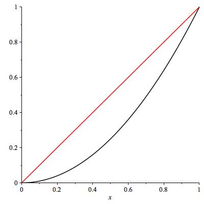
Let's compare \(x\) and \(x^2\) at \(x=0\text{.}\) At infinity, we know \(x \ll x^2\text{.}\) At zero, both go to zero but at possibly different rates. Have a look at Figure 7.18. You can see that \(x\) has a postive slope whereas \(x^2\) has a horizontal tangent at zero. Therefore, \(x^2 \ll x\) as \(x \to 0^+\text{.}\) You can see it from Figure 7.18 or from L'H{\^o}pital:
Example 7.19.
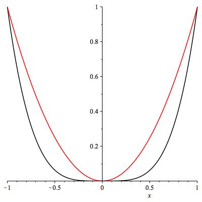
What about \(x^2\) and \(x^4\) near zero? Both have slope zero. By eye, \(x^4\) is a lot flatter. Maybe \(x^4 \ll x^2\) near zero. It is not clearly settled by the picture (do you agree? see Figure 7.20), but the limit is easy to compute.
Checkpoint 98.
Here is a less obvious example, still with powers.
Example 7.21.
Let's compare \(\sqrt{x}\) and \(\sqrt[3]{x}\) near zero. See Figure 7.22. Is one of these functions much smaller than the other as \(x \to 0^+\text{?}\) Here, the picture is pretty far from giving a definitive answer!
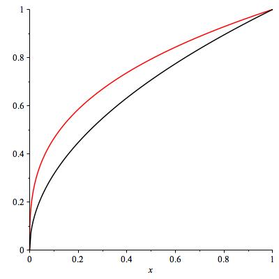
We try evaluating the ratio: \(f(x) / g(x) = x^{1/2} / x^{1/3} = x^{1/2 - 1/3} = x^{1/6}\text{.}\) Therefore,
and indeed \(x^{1/2} \ll x^{1/3}\text{.}\) Intuitively, the square root of \(x\) and the cube root of \(x\) both go to zero as \(x\) goes to zero, but the cube root goes to zero a lot slower (that is, it remains bigger for longer).
Checkpoint 99.
Let \(a,b,K,L\) be positive constants with \(a \lt b\text{.}\) Determine which of \(K x^a\) or \(L x^b\) is much greater than the other at \(x=0\text{,}\) if either.
\(\displaystyle Kx^a\ll Lx^b\)
\(\displaystyle Lx^b\ll Kx^a\)
both
neither
\(\text{Choice 2}\)
Suppose \(f\) and \(g\) are two nice functions, both of which are supposed to be approximations to some more complicated function \(H\) near the argument \(a\text{.}\) The question of whether \(f - H \ll g - H\text{,}\) or \(g - H \ll f - H\text{,}\) or neither as \(x \to a\) is particularly important because it tells us whether one of the two functions \(f\) and \(g\) is a much better approximation to \(H\) than is the other. We will be visiting this question shortly in the context of the tangent line approximation, and again later in the context of Taylor polynomial approximations.
"For sufficiently large \(x\)".
Often when discussing comparisons at infinity we use the term "for sufficiently large \(x\)". That means that something is true for every value of \(x\) greater than some number \(M\) (you don't necessarily know what \(M\) is). For example, is it true that \(f \ll g\) implies \(f < g\text{?}\) No, but it implies \(f(x) < g(x)\) for sufficiently large \(x\text{.}\) Any limit at infinity depends only on what happens for sufficiently large \(x\text{.}\)
Example 7.23.
We have seen that \(\ln x \ll \sqrt{x - 5}\text{.}\) It is not true that \(\ln 6 < \sqrt{6-5}\) (the corresponding values are about \(1.8\) and 1) and it is certainly not true that \(\ln 1 < \sqrt{1-5}\) because the latter is not even defined. But we can be certain that \(\ln x < \sqrt{x-5}\) for sufficiently large \(x\text{.}\) The crossover point is between 10 and 11.