Unit 5 Derivatives
Subsection 5.1 Concept of the derivative
It's easy to define your average speed for a trip: take the number of miles, divide by the number of hours, and there's your average speed in miles per hour. If you journey at constant speed, then that's also your speed at every moment of the trip. Most of us do not travel at constant speed. What is your speed then? How do you define it? How do you measure it? How do you compute it if you know some equation for your position at time \(t\text{?}\)
The concept of instantaneous speed is subtle. It is what spurred the invention of calculus over a few decades near the year 1700. It is a very general notion. Average speed is distance traveled per total time. Instantaneous speed is some instantaneous version.
Checkpoint 57.
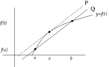
The figure shows distance traveled \((f(t))\)against time \((t)\text{.}\) The slope of line \(P\) can be interpreted as what in terms of speed? What about the slope of line \(Q\text{?}\)
If you replace "distance traveled" by "production price" and "time elapsed" by "units produced" you get the notions of average production cost per unit; marginal cost per unit is the instantaneous version. The list of applications is endless. Mathematically, they are all the same: if \(f\)is a function and \(x_0\)and \(x_1\)are starting and ending arguments for \(f\text{,}\) then the average change in \(f\)over the interval is \((f(x_1) - f(x_0)) / (x_1 - x_0)\text{;}\) the instantaneous rate of change of \(f\)with respect to \(x\)is called the derivative of \(f\) with respect to \(x\) and denoted \(f'(x)\text{.}\)
Checkpoint 58.
What is the tangent line to the graph of a linear function? (Hint: this is a so-easy-it’s-hard sort of question.)
Use your answer above to find \(f'(x)\) if \(f(x) = mx + b\text{.}\) \(f'(x)=\)
Undefined
In this section we will see how to understand \(f'\) both physically and mathematically. We will continue to use instantaneous speed as a running example of the physical concept, and instantaneous rate of change of \(f(x)\) with respect to \(x\) as the corresponding mathematical concept.
Remark 5.1.
We can take the slope of the function \(f\) at any point. Taking it at \(x\) gives a value we call \(f'(x)\text{.}\) That means that \(f'\) is a function: give it an argument \(x\)and it will produce the slope of \(f\) at that point. It will be helpful to keep in mind that the derivative operator takes as input functions \(f\) and produces as output their derivatives \(f'\text{.}\) Operator is a fancy word for a function whose input and output are functions rather than numbers. Taking derivatives is a linear operator. This is captured in Proposition 6.1 through Proposition 6.3 below.
Checkpoint 59.
Suppose you replace “distance traveled” by “elevation of trail” and “time elapsed” by “distance hiked”. What would be the physical interpretation of the instantaneous rate?
Subsection 5.2 Definitions
Most functions we use in mathematical modeling have unique tangent lines at most points. The slope of the tangent line to the graph of \(f\)at the point \((x,f(x))\) seems like one reasonable definition of \(f'(x)\text{.}\) In rare cases, such as you have already seen, we can use geometry to prove there is exactly one line tangent to the graph of \(f\)at a point and compute the slope.
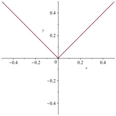
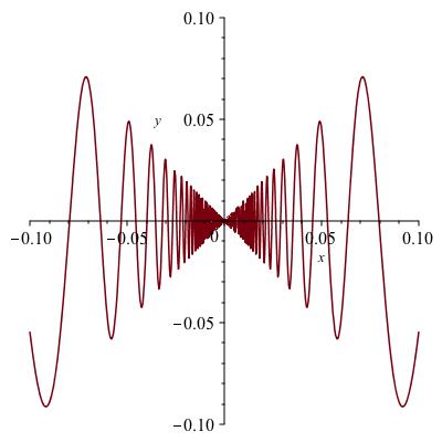
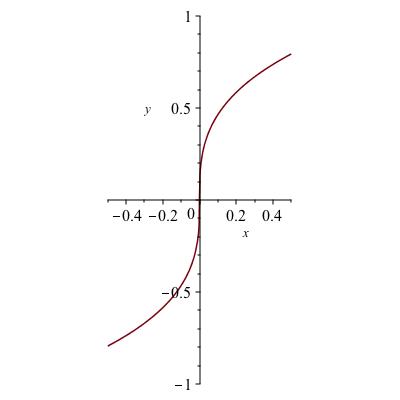
Unfortunately, there are not many functions for which the graph is a well known geometric object. In most cases we can't use geometry to conclude that there is a tangent line, that there is only one tangent line, or what the slope of this line is, if indeed there is exactly one. Keeping this in mind, we will use limits to come up with a definition that works for most functions and, when it does not work, as in the examples in Figure 5.2, gives an indication of why. In cases when it does not work, in fact we would probably agree that there is no good way to make sense of the instantaneous slope.
Checkpoint 60.
The graphs of \(|x|\text{,}\) \(x \sin (1/x)\)and \(\sqrt[3]{x}\)are shown in Figure 5.2. All contain the point \((0,0)\) provided we add zero to the domain of the second function and define the function to be zero there. In each case, say whether there is one, none, or more than one tangent line to the graph at \((0,0)\text{.}\)
\(|x|\text{:}\)
none
one
more than one
\(x\sin(1/x)\text{:}\)
none
one
more than one
\(\sqrt[3]{x}\text{:}\)
none
one
more than one
In which of these cases do you think there is a well defined slope of the tangent at \((0,0)\text{?}\)
\(|x|\text{:}\)
well-defined slope
no well-defined slope
\(x\sin(1/x)\text{:}\)
well-defined slope
no well-defined slope
\(\sqrt[3]{x}\text{:}\)
well-defined slope
no well-defined slope
We can take average slopes over any interval we want. The slope over the interval \([a,b]\) is the slope of the secant line passing through \((a,f(a))\) and \((b,f(b))\text{.}\) This is also called the difference quotient of \(f\) at the arguments \(a\) and \(b\text{.}\) What happens when one endpoint of the interval is \(x\) and the other is very close to \(x\text{?}\) Pictorially, it looks the slope get very close to the slope of the tangent line at \((x,f(x))\text{.}\) Figure 5.3 gives a tool for exploring this secant-line-to-tangent-line approximation.
Definition using limits.
The derivative is a mathematical definition meant to compute the slope of the tangent line at \(a\text{.}\) Definition 5.4, however, only talks about limits of slopes of secants, not of tangents. Do you think these two notions will always coincide? There isn't a right answer to this.
Checkpoint 61.
Do you think these two notions will always coincide?
Definition 5.4.
Let \(f\) be a function whose domain contains an interval around the point \(a\text{.}\) Define
if the limit exists, and say that \(f'(a)\)is undefined if the limit does not exist. Because we want to emphasize that \(b-a\)is going to zero, we often define \(h := b-a\)and rewrite the definition as
The two equations (5.1) and (5.2) are algebraically equivalent.
Checkpoint 62.
-
In Definition 5.4, which variables are free and which are bound?
\(a\text{:}\)
free
bound
\(b\text{:}\)
free
bound
\(f\text{:}\)
free
bound
\(h\text{:}\)
free
bound
-
In Figure 5.3, what values of \(a\)and \(b\) are being illustrated?
\(a=\)
\(b=\)
Suppose a student complains that Figure 5.3 illustrates a limit of the form \(\lim_{b \to a^+}\text{,}\) not \(\lim_{b \to a}\text{.}\) What could you add to the picture to address her concerns?
Example 5.5.
Let \(f(x) = x^2\text{.}\) Let's see the definition to try to compute \(f'(1)\text{.}\) By definition, this is
Evaluating the numerator gives
The first equality is true because we can cancel the factors of \(b-1\) (remember, the limit looks at values of \(b\) near 1 but not equal to 1). The second equality is true because we can evaluate the limit of the polynomial \(b+1\) at \(a=1\) by plugging in 1 for \(b\) (Proposition 4.30).
Checkpoint 63.
Let \(f(x) = x^2 + {2}\text{.}\) Compute \(f'({5})\) directly from the definition, as we did in the previous example.
\(f'({5})=\)
\(10\)
Notation.
We already agreed to use a prime after the function name as one way to denote a derivative. Thus the derivative of \(f\) is \(f'\text{,}\) the derivative of \(g\) is \(g'\text{,}\) the derivative of \(\Gamma\) is \(\Gamma'\text{,}\) etc. We may need to refer to the derivative of a function when it has not been given a name. One could imagine something like the notation \((cx)'\) for the derivative of the function "multiply by \(c\)", or perhaps the more precise \((x \mapsto cx)'\text{.}\)
To avoid ambiguity, we use the notation \(\frac{df}{dx}\)for the derivative of \(f\)with respect to \(x\text{.}\) This is better than \(f'\)when there is more that one variable that could be differentiated. that one variable that could be differentiated. You can also write this as \(\frac{d}{dx} f\)when \(f\)is a big long cumbersome expression, for example,
Then there is the question of how to write \(f'(a)\text{,}\) the value of the function \(f'\)at argument \(a\text{,}\) in this notation. Should we write \(\frac{d\, f(a)}{dx}\)or \(\frac{df}{dx} (a)\text{?}\) The second is better, for example, \(\frac{d(x^3-3x+1)}{dx} (a)\text{,}\) because the first looks like you are differentiating a constant. Another common way of writing this is \(\left. \frac{d \, (x^3 - 3x + 1)}{dx} \right|_{x=a}\text{.}\)
Checkpoint 64.
Suppose the number of feet an object has fallen after \(t\) seconds is given by \(16 t^2 + ct\) where \(c\) is its initial downward velocity (This is in fact true when air resitance is ignored and the earth’s gravitational constant is approximated.). Write an expression for the downward instantaneous speed of the object after \(t\) seconds. Please don’t compute any derivatives, just write an expression in some notation involving a derivative.
Now write an expression for the downward instantaneous speed of the object after \(s\) seconds.
\(\frac{d}{dt}\!\left(16t^{2}+ct\right)\)
Further interpretations: error propagation and marginal effect.
You have seen examples in which derivatives represent speed. More generally, the derivative of a function of time represents the rate of change of the quantity per time. Here are some other things derivatives commonly represent.
Suppose you have a formula \(f(x)\) involving a quantity \(x\) that is measured, but with measurement error. Then \(f'(x)\) tells you how much error you get in \(f\) per amount of error in measuring \(x\text{.}\)
Example 5.6.
A \(4 \times 8\) foot board is cut parallel to the long side to obtain a \(3 \times 8\) board. The accuracy of the cut is \(1/4\) inch. What is the accuracy of the area, in square feet? Writing \(A = \ell \times w\) and differentiating gives \(dA/dw = \ell =\)8 feet in our case. Therefore, the error in area (in square feet) is 8 feet times the measurement error in the width (in linear feet). Plugging in a measurement error of \(1/4\)inch, which equals \(1/48\) feet, we see the area is accurate to within \(8 \mbox{ ft} \times \frac{1}{48} \mbox{ ft} = \frac{1}{6} \mbox{ ft}^2 \text{.}\)
The symbol \(\Delta\) is the upper case Greek letter Delta an often used to denote change in a quantity or error in a measurement.
Checkpoint 65.
Let \(\Delta x\) denote the possible error in \(x\text{,}\) and \(\Delta f\)denote the possible resulting error in \(f(x)\text{.}\) Write a formula relating these quantities and the derivative of \(f\text{.}\)
Another interpretation is the marginal effect of the variable on the function. For example, if \(f(x)\) represents the cost of producing \(x\) barrels of refined oil, then \(f'(x)\) is the marginal cost of production of more oil. Unless \(f\) is linear, this will depend on \(x\text{.}\) The marginal cost of further production usually depends on the present level of production.
Subsection 5.3 First and second derivatives, and sketching
Knowledge of the deriviatve can help you sketch a function more accurately. The very first practice problem asked you to incorporate slope information into a sketch. Sketching is as much an art as a science, but there are methodical ways to use information about the function and its derivatives.
To begin with, knowing where the derivative is positive and negative determines whether it is sloping up or down as you move right. In other words, the sign of the derivative indicates whether the function is increasing or decreasing. Where the sign of the derivative changes from positive to negative as you move right, the function changes from increasing to decreasing. That means someone hiking on the graph of the function from left to right has been walking upwards and now begins to walk downward; see Figure 5.7.
Checkpoint 66.
What does the hiker’s landscape look like if \(f'\) is negative to the left of the value \(x=a\) and positive to the right?
Because transitions in the sign of \(f'\)correspond to hilltops and valley floors, finding values of \(x\)that are maxima and minima for \(f(x)\) involves finding values of \(x\)for which \(f'(x) = 0\text{.}\) We discuss this at greater length in Unit 8. For the purposes of sketching, the moral of the story is: know where \(f'\) is positive and where it is negative, and use this to depict a function that is increasing and decreasing in the right places.
Checkpoint 67.
Sketch the graph of a function \(f\) such that \(f'\) is positive when \(x \lt 1\text{,}\) dips to zero at \(x=1\text{,}\) is positive again until \(x=3\text{,}\) is zero at \(x=3\text{,}\) and is negative to the right of \(x=3\text{.}\) See if you can also make \(f\) have a unique zero at \(x = -2\text{.}\)
The second derivative.
A Japanese proverb says, "The other side also has another side." The function \(f\) has a derivative. \(f'\) is also a function. Therefore, The derivative also has a derivative. Not quite so poetic, but very useful for sketching functions. The derivative of the derivative is called the second derivative, denoted \(f''\text{,}\) or \(\frac{d^2 \, f}{dx^2}\text{.}\) The sign of the derivative says where a function is increasing or decreasing, therefore the sign of \(f''\) indicates where the slope \(f'\) is increasing or decreasing. We use italics here as a visual reminder that there are a number of levels (original function, first derivative, second derivative) and attributes (positive/negative, increasing/decreasing) and it's easy to get mixed up what corresponds to what. We hope Table 5.8 helps clarify whose positivity says what about whom.
| \(f''\) is | \(f'\) is | \(f\) is | graph of \(f\) |
| positive | increasing | of increasing slope | concave upward |
| negative | decreasing | of decreasing slope | concave downward |
| positive | increasing | upward | |
| negative | decreasing | downward | |
| positive | above the horizontal axis | ||
| negative | below the horizontal axis |
Remark 5.9.
The placement of the 2 in the numerator of \(\frac{d^2 \, f}{dx^2}\) may seem strange, but it reflects something important: \((d/dx)\) is a differential operator, and \((d^2 / dx^2)\) is the result of applying this operator twice. This becomes important in later courses such as Math 114.
Checkpoint 68.
Let \(g(x) := x^2\text{.}\) Compute \(g'' (x)\text{.}\)
\(2\)
Of course, not every function is differentiable, and not every derivative is itself differentiable, so \(f''\) may not exist even if \(f'\) exists.
We have talked informally about functions that are concave up or down. It is time to give a definition. In fact we give two definitions, one algebraic and one pictorial. The pictorial one is in fact more general because it works when \(f'\) does not exist. When \(f'\) exists on \((a,b)\text{,}\) then the two definitions agree.
Definition 5.10. concavity.
When the function \(f'\) exists and is increasing, we say that \(f\) is concave upward.
When the function \(f'\) exists and is decreasing, we say that \(f\) is concave downward.
Definition 5.11. concavity (pictorial definition).
If \((a,b)\)is an open interval in the domain of \(f\)and if for every pair of numbers \(x,y \in (a,b)\)the graph of \(f\)on \((a,b)\) lies below the line segment connecting \((x,f(x))\)to \((y,f(y))\text{,}\) we say that \(f\) is concave upward on \((a,b)\text{.}\)Checkpoint 69.
If \(f''\)exists and is positive, can you conclude anything about concavity of \(f\text{?}\)
How about if \(f''\) exists and is negative?
To summarize, if \(f''\) exists on \((a,b)\) then the sign of \(f''\) determines the concavity of \(f\text{.}\) If \(f''\) doesn't exist or you can't compute it, use Definition 5.10 Definition 5.11.
Points of inflection.
We never formally defined a tangent line. One definition would be "A line that touches a graph of a function at precisely one point and stays on one side of the graph other than this."
Checkpoint 70.
Here are four ways this definition may fail to capture what some people think a tangent line should be. For each example, please say whether you think the given line ought to count as a “tangent line.”
-
Graph of \(y = |x|\text{;}\) any line with absolute slope less than 1.

is a tangent line
is not a tangent line
-
Graph of \(y = \tan x\text{;}\) line of slope 1 through the origin.

is a tangent line
is not a tangent line
-
Graph of a cubic with a tangent line that intersects the cubic elsewhere.

is a tangent line
is not a tangent line
-
Graph with a vertical cusp.

is a tangent line
is not a tangent line
\(\text{is a tangent line}\hbox{ or }\text{is not a tangent line}\)
\(\text{is a tangent line}\hbox{ or }\text{is not a tangent line}\)
\(\text{is a tangent line}\hbox{ or }\text{is not a tangent line}\)
\(\text{is a tangent line}\hbox{ or }\text{is not a tangent line}\)
As you can see, the intuitive definition of tangent line is subject to unanticipated judgment calls. This motivates a more formal definition.
Definition 5.12. tangent line.
If \(f\)is differentiable at \(a\text{,}\) the tangent line to \(f\) at \(a\) is defined to be the line \((y-f(a)) = m (x-a)\) where \(m = f'(a)\text{.}\)
Checkpoint 71.
Is the point \((a,f(a))\) always on the tangent line to \(f\) at \(a\text{?}\)
yes
no
Explain why or why not.
\(\text{yes}\)
One confusing case is when the second derivative is zero. What happens to the concavity at such a point? Often it switches from up to down or vice versa. Wherever concavity switches is called a point of inflection. The geometric concept of an inflection point does not require calculus, though the notion seems not to have been discussed much before the advent of calculus.
Checkpoint 72.
Which of the graphs in Checkpoint 5.14 shows a point of inflection?

inflection point
no inflection point

inflection point
no inflection point

inflection point
no inflection point

inflection point
no inflection point
Checkpoint 73.
- Sketch a graph of the sine function.
- Mark the intervals where sine increases and those where it decreases.
- On the same graph sketch the cosine function.
- The derivative of \(\sin\) is \(\cos\text{;}\) what does this imply about the values of cosine on the marked intervals?
- Where are the points of inflection for sine and what happens to the cosine at those arguments?