Unit 1 Approximations and bounds
This e-textbook is about using math for modeling and coming up with plausible analyses. One of the course goals is number sense. Wikipedia defines this as "an intuitive understanding of numbers, their magnitude, relationships, and how they are affected by operations."
Example 1.1. Food for thought.
If you have a model for spread of disease where the number of infections doubles every three days, how long can this go on before the model has to change: A few years? A few months? A few weeks? A few days?
If some kind of answer began to form in your mind without your stopping to get out a calculator, then you have some of the ingredients of number sense already: perhaps you understand exponential growth, perhaps you can remember about how many people there are in the country or the world, perhaps you are familiar with powers of two and know how they relate to this problem. It is useful to be able to think this way. It's not important whether you use a calculator to answer any given question, but realistically, how often will you stop in casual conversation and whip out a calculator?
In this course, we'll teach you a number of these ingredients: use of logs, converting to powers of ten, tangent line approximation, Taylor polynomials, pairing off positive and negative summands, approximating integrals with sums and vice versa. Discussions of these will be brief. The point is to use them when you need them, which turns out to be nearly every lesson.
Today we're going to start with the tangent line approximation. You might think this odd because we haven't taught you calculus yet. Calculus is a way of computing the slopes of tangent lines to graphs. But conceptually, understanding the tangent line approximation takes knowledge only of algebra and geometry, not calculus. So, we'll preview the idea now, and in fact several more ideas from the course, and then later see how to use calculus to do these analyses more methodically.
Subsection 1.1 Where should I put my ladder?
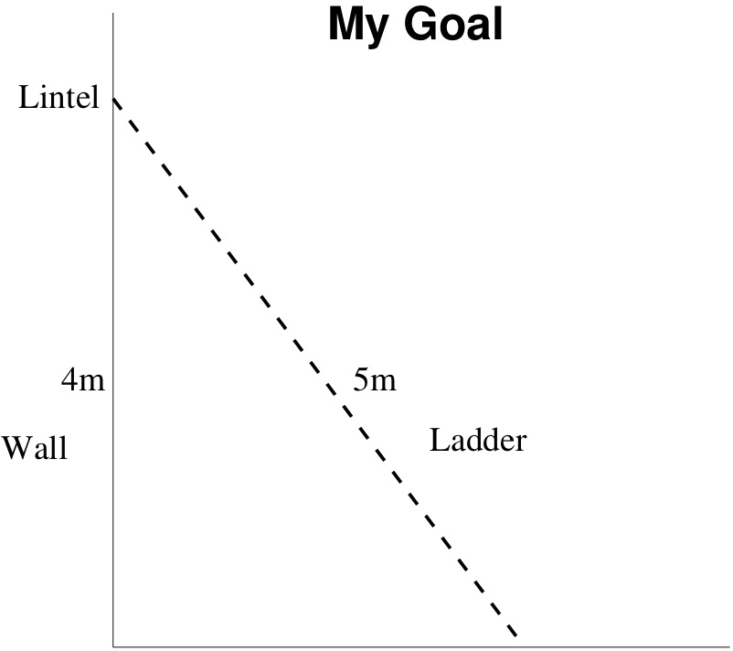
I am hanging wind chimes on my balcony using a ladder 5 meters long. On the highest safe step, my shoulders will be exactly at the top of the ladder, which I need to be at the height of the balcony rail, 4 meters above the ground. Every time I reposition the ladder I scratch the paint, so I'd rather not move it too many times. I need to get my shoulders within a couple of centimeters of the right height in order to drive a nail into the lintel. Where should I put the base of the ladder? The Pythagorean theorem tells me the it should be 3 meters from the wall; see Figure 1.2
Unfortunately, I didn't measure right, maybe because of the bulge at the bottom of the balcony. I am 20 cm too low. Now what? Solution: Let \(h\) be the function representing the height of the ladder as a function of the position of the base, in other words, \(h(x)\) is the height of the ladder on the wall (in meters) when the base is \(x\) meters from the wall. By the Pythagorean Theorem, \(h(x) = \sqrt{25 - x^2}\text{.}\)
The height I am trying to reach is shown in Figure 1.3. which has \(x=3\) and \(h(x) = 4\text{.}\) Instead I hit some other point \(z\) with \(h(z) = 3.8\text{.}\) Clearly \(z\) is too far from the wall. How far do I need to scoot the ladder toward the wall? As you can see in Figure 1.3, due to the balcony and the hedge, it was not feasible to measure either the height of the lintel or the distance I placed the foot of the ladder more accurately.
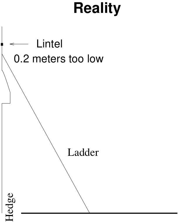
Figure 1.4 shows the graph of \(h\) and a tangent line to the graph of \(h\) at the point \((3,4)\text{.}\) The tangent line is a very good approximation to the graph near \((3,4)\text{.}\) For values of \(x\) between perhaps 2.6 and 3.4, the line is still visually indistinguishable form the graph.
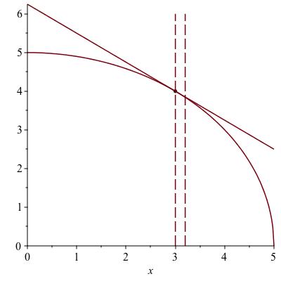
If we know the slope of this line, \(m\text{,}\) we can write the equation of the line: \((y-4) = m (x-3)\text{.}\) Because \(h(x)\) is very nearly equal to this \(y\) (because the curve nearly coincides with the line), we can write \(h(x) \approx 4 + m(x-3)\text{.}\) The wiggly equal sign is not a formal mathematical symbol. Here, it means the two will be close, but has no guarantee of how close, and furthermore, it is only supposed to be close when \(x\) is close to \(3\text{.}\) This is called an {\bf estimate}. Shortly, we will talk about bounds: estimates that do come with guarantees.
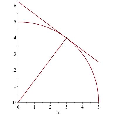
What is the slope of this line? The graph is a quarter-circle. Recall from geometry that any tangent to a circle makes a right angle with the radius. The slope of the radius from \((0,0)\) to \((3,4)\) is \(s = 4/3\text{.}\) The slope of any line making a right angle with this is the negative reciprocal \(-1/s = - 3/4\text{.}\) In other words, the slope of the tangent line is \(-3/4\text{.}\)
Checkpoint 1.
Approximately what distance must the foot of the ladder be scooted back toward the house?
\(0.27\)
We need to make up a gap of 20 centimeters, or .2 meters. Approximately, the height of the end of the ladder changes by \(-3/4\) meter for each meter we move the base of the ladder. So we need to solve
where \(Delta\) is the amount we move the base of the ladder. Thus \(\Delta=\frac{.2}{-\frac{3}{4}}=.2666\cdots\text{.}\)
The reason we chose this particular example to demonstrate the tangent line approximation is that we could compute the slope with high school geometry. With calculus, we'll be able to find the slope of a tanget line to just about any function we can think of. In fact the word calculus when it was invented meant literally "a method of computing".
Checkpoint 2.
The tangent line estimate for \(\sqrt{x}\) near \(x=9\) is given by
which we might write as
Which of these best caputes the meaning of this symbolic expression?
\(\sqrt{x}\) will be closer to \(3 + \frac{x-9}{6}\) than \(x\) is to 9.
The closer \(x\) gets to 9, the closer \(\sqrt{x}\) will be to \(3 + \frac{x-9}{6}\text{.}\)
\(3 + \frac{x-9}{6}\) is the best approximation for \(\sqrt{x}\) when\(x\) is near 9.
There is no well defined meaning, it's just an intuitive statement.
\(\text{Choice 2}\)
Subsection 1.2 Bounding
To get an upper bound on \(f(x)\) means to find a quantity \(U(x)\) that you understand better than \(f (x)\) and for which you can prove that \(U(x) \geq f(x)\text{.}\) A lower bound is a quantity \(L(x)\) that you understand better than \(f(x)\) and that you can prove to satisfy \(L(x) \leq f(x)\text{.}\) If you have both a lower and upper bound, then \(f(x)\) is stuck for certain in the interval \([L(x),U(x)]\text{.}\)
Checkpoint 3.
While estimating produces statements that are not mathematically well defined, bounding produces inequalities with precise mathematical meaning. Two ways we typically find bounds are as follows.
First, if \(f\) is monotone increasing then an easy upper bound for \(f(x)\) is \(f(u)\) for any \(u \geq x\) for which we can compute \(f(u)\text{.}\) Similarly an easy lower bound is \(f(v)\) for any \(v \leq x\) for which we can compute \(f(v)\text{.}\) If \(f\) is monotone decreasing, you can swap the roles of \(u\) and \(v\) in finding upper and lower bounds. There are even stupider bounds that are still useful, such as \(f(x) \leq C\) if \(f\) is a function that never gets above \(C\text{.}\)
Example 1.6. An Unexample.
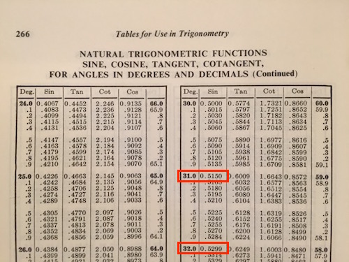
Suppose we wanted to estimate \(\sin (1)\text{.}\) The easiest upper and lower bounds are \(1\) and \(-1\) respectively because \(\sin\) never goes above \(1\) or below \(-1\text{.}\) A better lower bound is \(0\) because \(\sin (x)\) remains positive until \(x=\pi/2\) and obviously \(1 \lt \pi/2\text{.}\) You might in fact recall that one radian is just a bit under \(60^\circ\text{,}\) meaning that \(\sin (60^\circ) = \sqrt{3}/2 \approx 0.0866\ldots\) is an upper bound for \(\sin (1)\text{.}\) Computing more carefully, we find that a radian is also less than \(58^\circ\text{.}\) Is \(\sin (58^\circ)\) a better upper bound? Probably not: we don't know how to calculate it, so it's not a quantity we understand better. Of course is we had an old-fashioned table of sines, and all we can remember about one radian is that it is between \(57^\circ\) and \(58^\circ\text{,}\) then \(\sin (58^\circ)\) is not only an upper bound but the best one we have.
Checkpoint 4.
Is the tangent line estimate in the ladder problem an upper bound, a lower bound, both, or neither?
an upper bound
a lower bound
both
neither
Explain.
\(\text{an upper bound}\)
Subsection 1.3 Concavity
A more subtle bound come when \(f\) is known to be concave upward or downward in some region. By definition, a concave upward function lies below its chords and a concave downward function lies above its chords.
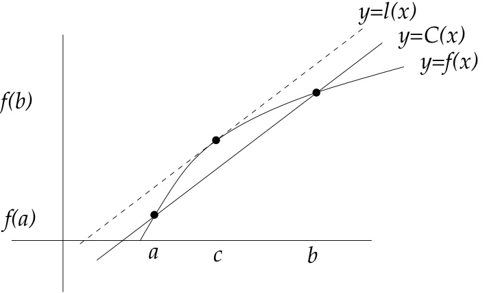
Figure 1.8 shows a function \(f(x)\) which is concave down. As long as \(x\) is in the interval \([a,b]\text{,}\) we are guaranteed to have \(C(x) \leq f(x)\text{.}\) On the other hand, when \(f'' \lt 0\) on an interval, the function always lies below the tangent line. Therefore \(L(x)\) is an upper bound for \(f(x)\) when \(x \in [a,b]\) no matter which point \(c \in [a,b]\) at which we choose to take the linear approximation.
In the ladder example, we were lucky that the graph was a familiar geometric shape, a quarter circle, which we know to be convex. We are able to conclude that the tangent line remains above the graph because we know geometrically that the tangent line to a circle touches the circle at one point and otherwise remains outside the circle. Calculus will give us a far more general way to determine concavity.
Checkpoint 5.
It turns out that the square root function is concave downard. What does this tell you about the estimate
This approximation is an upper bound.
This approximation is a lower bound.
This approximation is both an upper and a lower bound.
This approximation is neither an upper nor a lower bound.
\(\text{This approximation ... bound.}\)