Unit 15 Taylor approximations
We started the course (back in Unit 1) with the idea of approximating a function \(f(x)\) by its tangent line. The problem of actually finding the tangent line is what motivated us to think hard about limits and how they work, then to apply that idea to secant lines.
Here's another definition of the tangent line (in addition to the ones we saw in Subsection 5.2):
Definition 15.1. alternative definition of the tangent line.
The tangent line to the graph of \(f(x)\) at \(x=c\) is the graph of the linear function \(L(x)=mx+b\) which is as good an approximation to \(f(x)\) nearby to \(x=c\) as any linear function can be.This definition might make you a bit uncomfortable. How would you use this definition to actually find a tangent line?
We'll use the notion of asymptotic equivalence from Subsection 7.3. What we'd like, first of all, is that \(f(x)\sim L(x)\) as \(x\to c\text{.}\) In other words, we want
Now as long as \(f(x)\) and \(L(x)\) are both continuous, and \(L(c)\neq 0\text{,}\) the rules of limits tell us that \(\lim_{x\to c}\frac{f(x)}{L(x)}=\frac{f(c)}{L(c)}\text{.}\) So we need \(\frac{f(c)}{L(c)}=1\text{,}\) which is just the requirement that \(L(c)=f(c)\text{.}\) For reference later, we'll say that the value \(f(c)\) approximates the function \(f(x)\) to zeroth order.
A line is determined by two pieces of information:
- a slope \(m\) and an intercept \(b\)
- a slope \(m\) and a point \((x_0,y_0)\) on the line
- two points \((x_0,y_0)\) and \((x_1,y_1)\) on the line
We just learned that the point \((c,f(c))\) has to be on the line we're looking for, so let's work with the second option and determine \(L\) by finding its slope.
Imagine a competition among all lines which pass through the point \((c,f(c))\text{,}\) for which one is "most like" \(f(x)\) nearby \(x=c\text{.}\) Using the point-slope form of the equation for a line, we know that any such competitor has to look like \(L(x)=f(c)+m(x-c)\text{.}\) Now:
All \(f(x)-f(c)\sim m(x-c)\text{ as }x\to c\) means is that
which can only happen if \(m=\lim_{x\to c}\frac{f(x)-f(c)}{x-c}=f'(c)\text{.}\)
In other words, this approach (finding an asymptotically-equivalent line) gives the same formula for the slope of the tangent line that we know and love.
You might ask: why all the work just to get the same formula? Because the understanding of the tangent line as "the line that matches \(f(x)\) near \(x=c\) as well as any line can" will generalize to questions like:
- What parabola matches the graph of \(f(x)\) near \(x=c\) as well as any parabola can?
- What cubic function approximates \(f(x)\) near \(x=c\) the best among all cubic functions?
- etc.
These polynomial approximations are known as the Taylor polynomials for \(f(x)\text{.}\) They allow you to use your knowledge of polynomials -- which you've no doubt spent many years honing -- to understand how nonpolynomial functions behave.
Subsection 15.1 Taylor polynomials
Start with a function \(f(x)\text{.}\) Our goal will be to figure out the best approximation of \(f(x)\) (near \(x=c\)) by a polynomial of whatever degree we want (call that degree \(n\)).
\(n=1\).
When \(n=1\text{,}\) we want a degree-1 polynomial approximation. That is, we want the tangent line. So we use
\(n=2\).
A degree-2 polynomial looks like \(q(x)=Ax^2+Bx+C\text{.}\) Since we're interested in what happens when \(x\to c\text{,}\) let's rewrite this form as \(q(x)=a_2(x-c)^2+a_1(x-c)+a_0\text{.}\) (The exact relationship between \(A,B,C\) and \(a_0,a_1,a_2\) isn't important -- we just want to make sure that we're writing everything in terms of \(c\text{.}\))
Let's again write down our demands. We want \(f(x)\sim q(x)\text{ as }x\to c\text{,}\) i.e.,
As \(x\to c\text{,}\) \(x-c\to 0\text{.}\) So \(\lim_{x\to c} q(x)=a_0\text{.}\) As long as \(f\) is continuous, \(\lim_{x\to c}f(x)=f(c)\text{.}\) So we need \(a_0=f(c)\text{.}\)
As we did in the linear case, let's imagine a competition among all quadratic polynomials of the form \(q(x)=a_2(x-c)^2+a_1(x-c)+f(c)\text{.}\) We demand:
But \(f(x)-f(c)\sim a_2(x-c)^2+a_1(x-c)\text{ as }x\to c\) just means
We can rearrange the fraction to:
As \(x\to c\text{,}\) \(\frac{1}{a_2(x-c)+a_1}\to\frac{1}{a_1}\text{.}\) We end up with \(a_1=f'(c)\text{.}\)
So now we know that \(q(x)=a_2(x-c)^2+f'(c)(x-c)+f(c)\text{.}\) Let's rewrite our demands again:
This means we need
The form of this limit is \(\frac{0}{0}\text{,}\) so we can apply L'Hôpital's Rule. We need to be a bit careful to differentate with respect to \(x\). The numerator's derivative is
and the denomator's is
Applying L'Hôpital's Rule, we get
So \(a_2=\frac{1}{2}f''(c)\text{.}\)
That is, the quadratic which best approximates \(f(x)\) near \(x=c\) is
\(n=3\).
Now let's approximate \(f(x)\) by a cubic of the form \(q(x)=a_3(x-c)^3+a_2(x-c)^2+a_1(x-c)+a_0\text{.}\) It probably won't surprise you that \(a_0=f(c)\text{.}\) Let's see about \(a_1\text{:}\)
which just means
or in other words
Because \(\frac{1}{a_3(x-c)^2+a_2(x-c)^+a_1}\to\frac{1}{a_1}\) as \(x\to c\text{,}\) we see that \(a_1=f'(c)\text{.}\)
So now we have
In order words, we need
L'Hôpital tells us that
So \(a_2=\frac{1}{2}f''(c)\text{.}\)
Let's update our demand:
So we consider the limit
Again L'Hôpital's Rule applies here, so we differentiate the numerator and the denominator to get:
This form is still indeterminate, so we apply L'Hôpital's Rule again:
Thus, we need to use \(a_3=\frac{1}{6}f'''(c)\text{.}\) Our approximating cubic is therefore:
Let's write these out so that we can see the pattern.
Can you see the pattern?
Checkpoint 180.
The last term of \(T_4(x)\) will look like
where the something is .
\(24\)
Definition 15.2. Taylor polynomials.
The degree-\(n\) Taylor polynomial for \(f(x)\) at \(x=c\) is
A few observations to help you remember this formula:
- The variable here is \(x\) -- not \(c\text{.}\)
- In the formula for \(T_n\text{,}\) the derivatives of \(f\) are all evaluated at \(x=c\).
- In each term, there is a derivative, a power of \(x-c\text{,}\) and a factorial. These all share the same index.
- \(T_3(x)\) is just \(T_2(x)\) plus a term of degree 3; \(T_4(x)\) is just \(T_3(x)\) plus a term of degree 4; etc.
Example 15.3.
Compute the degree-4 Taylor polynomial for \(f(x)=\sin(x)+\cos(x)\) at \(x=\frac{\pi}{6}\text{.}\)
First, we'll need to compute some derivatives:
The formula in Definition 15.2 then yields:
Now you try your hand at it:
Checkpoint 181.
Compute the degree-3 Taylor polynomial for \(f(x)=\sqrt{x}\) near \(x=4\text{.}\)
\(2+0.25\!\left(x-4\right)-0.015625\!\left(x-4\right)^{2}+0.00390625\!\left(x-4\right)^{3}\)
Here's another important property of the Taylor polynomials.
Checkpoint 182.
Differentiate the degree-4 Taylor polynomial at \(x=c\text{;}\) that is, compute
and evaluate at \(x=c\text{.}\) What do you get?
Now compute the further derivatives at \(x=c\text{:}\)
\(\frac{d^2}{dx^2}|_{x=c}T_4(x)=\)
\(\frac{d^3}{dx^3}|_{x=c}T_4(x)=\)
\(\frac{d^4}{dx^4}|_{x=c}T_4(x)=\)
\(\frac{d^5}{dx^5}|_{x=c}T_4(x)=\)
This exercise shows two things:
- where the factorial comes from in each term of the Taylor polynomial
- that the derivatives of the Taylor polynomial are the same as the derivatives of \(f\text{,}\) at least at \(x=c\)
Definition 15.4. Maclaurin polynomials.
When we use \(c=0\text{,}\) we call the result the Maclaurin polynomials.Example 15.5.
Let's compute the degree-5 Maclaurin polynomial for \(f(x)=e^x\text{:}\)
So the Maclaurin polynomial is
Subsection 15.2 Taylor and Maclaurin polynomials in graphing
We claimed that the Taylor polynomials are polynomials that "act like" the function \(f(x)\) near \(x=c\text{.}\) What does that mean in terms of the graph of \(f(x)\) and its Taylor polynomials?
The fact that the graphs of the Taylor polynomials are similar to those of the original function \(f\) gives us a way to explain why the techniques mentioned in Subsection 5.3 work. Let's imagine the situation of a function \(f(x)\) with \(f(1)=1\text{,}\) \(f'(1)=-\frac{1}{2}\text{,}\) and \(f''(1)=3\text{.}\) This is enough information to compute that the degree-2 Taylor polynomial at \(x=1\) is
Since the graph of \(T_2\) is close to the graph of \(f\text{,}\) we can infer properties of \(f\) from those of \(T_2\text{.}\)
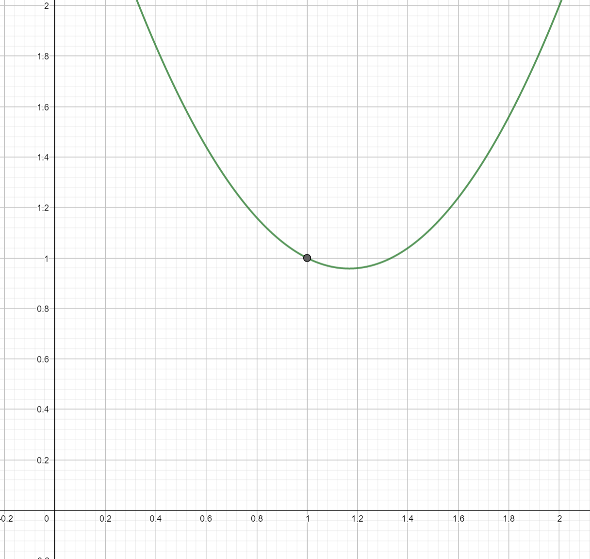
In particular, we know that any quadratic with a positive coefficient of \(x^2\) has a graph which is an upward-facing parabola. We conclude that \(f\) is concave-up near \(x=1\text{.}\)
This idea also tells us how to graphically interpret higher derivatives: a function with \(f'''(c)>0\) acts like a cubic with positive leading coefficient; one with \(f^{(4)}(c)\lt 0\) acts like a quartic with a negative leading coefficient; etc.
Example 15.8.
We want to hand-draw a precise graph of the cosine function near \(x=0\text{.}\)
The first approach might be to compute some values of cosine near \(x=0\text{,}\) say \(\cos(-.1)\text{,}\) \(\cos(-.2)\text{,}\) \(\cos(.1)\text{,}\) etc. But those are hard to do by hand! So instead, we'll use a function we know how to compute the values of by hand: the Maclaurin polynomial of degree 2. That's
The values of \(T_2\) are pretty straightforward to compute:
\(x\)
\(T_2(x)\)
\(-.6\)
\(1-\frac{1}{2}(-.6)^2=.82\)
\(-.4\)
\(1-\frac{1}{2}(-.4)^2=.92\)
\(-.2\)
\(1-\frac{1}{2}(-.2)^2=.98\)
\(0\)
\(1\)
\(.2\)
\(1-\frac{1}{2}(.2)^2=.98\)
\(.4\)
\(1-\frac{1}{2}(.4)^2=.92\)
\(.6\)
\(1-\frac{1}{2}(.6)^2=.82\)
Checkpoint 183.
In the example above, we used the degree-2 Maclaurin polynomial for \(f(x)=\cos(x)\text{.}\) Compute the degree-6 Maclaurin polynomial for \(f(x)=\cos(x)\text{.}\)
\(1-0.5x^{2}+0.0416667x^{4}-0.00138889x^{6}\)
Subsection 15.3 Computing Taylor Polynomials
There's always at least one way to compute a Taylor polynomial: use the formula in Definition 15.2. But that usually involves taking a lot of derivatives, which might not be so helpful if the function in question is complicated. So instead, we're going to approach the computation of Taylor polynomials the way we approached computing derivatives and integrals: list out the Taylor polynomials for some basic functions, and then state some rules for how the Taylor polynomial of a complicated function is related to those of its parts.
The basic idea behind all these rules is: Taylor polynomials are polynomials -- so you can do all of the lovely algebra to them that you learned in middle and high school.
| \(f(x)\) | Maclaurin polynomial of degree 4 |
| \(e^x\) | \(1+x+\frac{1}{2}x^2+\frac{1}{6}x^3+\frac{1}{24}x^4\) |
| \(\sin(x)\) | \(x-\frac{1}{6}x^3\) |
| \(\cos(x)\) | see Checkpoint 183 |
| \(\frac{1}{1-x}\) | \(1+x+x^2+x^3+x^4\) |
| \(\frac{1}{1+x}\) | \(1-x+x^2-x^3+x^4\) |
| \(\ln(1+x)\) | \(x-\frac{1}{2}x^2+\frac{1}{3}x^3-\frac{1}{4}x^4\) |
Simple Compositions.
Let's say we want to compute the degree-8 Maclaurin polynomial for \(f(x)=\sin(x^2)\text{.}\) We could go ahead and differentiate 8 times. But to save ourselves some work, let's switch variables. Set \(t=x^2\text{.}\) Table 15.10 tells us that
and that this is the best approximation by a polynomial which is degree 4 in \(t\text{.}\) Notice that being degree 4 in \(t\) is the same as being degree 8 in \(x\text{.}\) If we substitute \(t=x^2\) back into our polynomial, we get:
which is our answer.
This trick works with powers of \(x\) and multiples of \(x\text{.}\) For example, the degree-5 Maclaurin polynomial for \(f(x)=e^{3x}\) is
We can also do this with shifts: the degree-3 Maclaurin polynomial for \(\ln(2+x)=\ln(1+(x+1))\) is
Products.
Let's say we want to compute the degree-6 Maclaurin polynomial for the function \(h(x)=e^x\sin(x)\text{.}\) To use the formula in Definition 15.2, we would have to take sixth derivatives. Because of the product rule, \(h'(x)\) will have two terms; \(h''(x)\) will have four terms; etc. So that seems like kind of a mess. On the other hand, Table 15.10 tells us that
The Taylor polynomials are polynomials, so let's treat them like polynomials and multiply!
Checkpoint 184.
Let's go ahead and do the multiplication. I've color-coded the terms coming from \(e^x\) to help with the bookkeeping.
I've left off the remaining rows; you are an expert at manipulating polynomials so you can complete them yourself. But I want to point something out here: there are lots of terms with degrees greater than 6. Because we want a polynomial of degree 6, we can just omit these.
Checkpoint 185.
What is the degree-6 Maclaurin polynomial for \(e^x\sin(x)\text{?}\)
\(x+x^{2}+0.333333x^{3}+0x^{4}+-0.0333333x^{5}+-0.0111111x^{6}\)
More Complicated Compositions.
We can also use it with more complicated compositions such as \(f(x)=\cos(e^x-1)\text{.}\) Let's find the degree-3 Maclaurin polynomial for \(\cos(e^x-1)\text{.}\) We start with the degree-3 Maclaurin polynomial for \(\cos(t)\text{,}\) applied with \(t=e^x-1\text{:}\)
Now, we remind ourselves that \(e^x\approx 1+x+\frac{1}{2}x^2+\frac{1}{6}x^3\text{,}\) so that \(t=e^x-1\sim x+\frac{1}{2}x^2+\frac{1}{6}x^3\text{,}\) and make that substitution:
Like we did with products, now we bite the bullet and do the algebra:
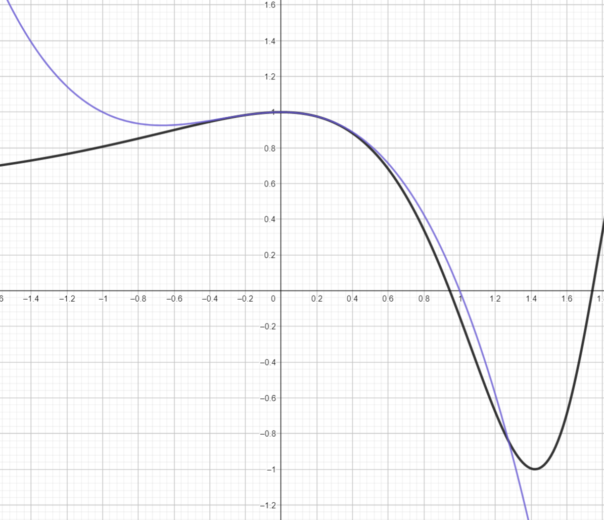
Notice that we actually got a degree 6 polynomial. Since we only needed to approximate \(f\) to order 3, we take the cubic part and our answer is:
Plotting \(T_3\) together with \(f\) confirms that this is a good approximation, at least near \(x=0\text{:}\)
Subsection 15.4 The Mean Value Theorem and Taylor's Theorem
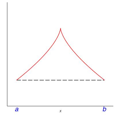
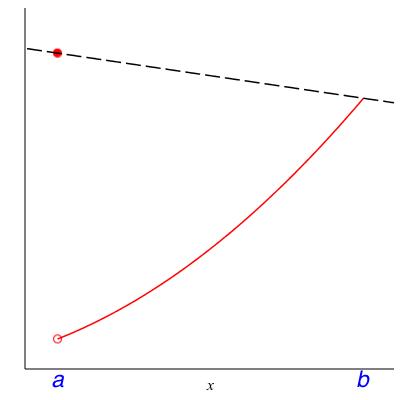
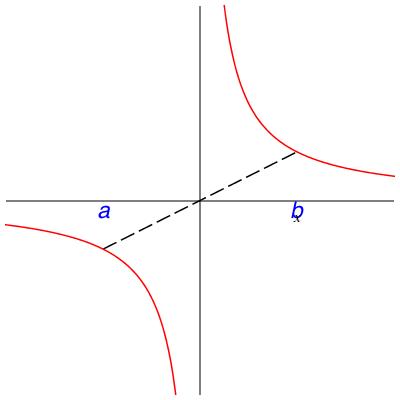
In class we will discuss the following theorem. Please read it now to see whether it makes intuitive sense to you. The hypotheses will be filled in after the class discussion centered on the counterexamples in Figure 15.12.
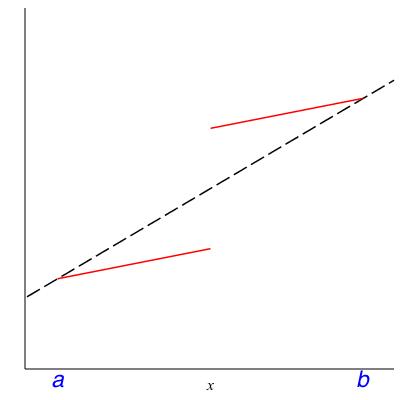
Theorem 15.13. Mean value theorem.
Let \(f\) be a function and \(a < b\) be real numbers. Assuming SOME HYPOTHESES there must be a number \(c \in (a,b)\) where the slope of \(f\)is equal to the average slope over \((a,b)\text{,}\) that is,Checkpoint 186.
What are some ways to fill in the SOME HYPOTHESES that make the Mean Value Theorem true? That is, what assumptions can we place on \(f\) which rule out the behavior in Figure 15.12?
Example 15.14.
Let \(f(x)\) be the position (mile marker) of a PA Turnpike driver at time \(x\text{.}\) Suppose the driver entered the Turnpike at Mile 75 (New Stanton) at 4pm and exited at Mile 328 (Valley Forge) at 7pm. What does the Mean Value Theorem tell you in this case? The average slope of \(f\) over interval \([4pm,7pm]\) is the difference quotient \((f(7) - f(4))/(7-4) = (325 - 75) / 3 = 83 \frac{1}{3}\text{.}\) Thus there is some time \(c\) between 4pm and 7pm that \(f'(c) = 83 \frac{1}{3}\) MPH, in other words, that this driver was traveling at a speed of \(83 \frac{1}{3}\) MPH.
Checkpoint 187.
In Example 15.14, the speed in question is above the posted speed limit along the Turnpike, 70 MPH.
Should this driver receive a speeding ticket? Give a mathematical argument for each side -- don't rely on mercy, or ``everybody does it", or things like that.
Example 15.15.
Let \(f(x) := 1/x\) and let \(a < b\) be positive real numbers. What, explicitly in terms of \(a\) and \(b\text{,}\) is the number \(c\) guaranteed by the Mean value theorem?Actually, Example 15.15 is a bit beside the point. The Mean Value Theorem only asserts that there is some number \(c\); it says nothing about what \(c\) actually is.
Why is the Mean Value Theorem in this chapter? We can rewrite (15.1) to read:
which looks an awful lot like the linear approximation to \(f\) at \(x=a\text{:}\)
except we've plugged in \(x=b\) and the place we're evaluating \(f'\) is different.
It turns out, this same sort of theorem is true for the higher-order polynomial approximations, too:
Theorem 15.16. Taylor's Theorem.
Let \(f\) be a function and \(a < b\) be real numbers. Assuming SOME HYPOTHESES, there must be a number \(c \in (a,b)\) whereCheckpoint 188.
The Mean Value Theorem is just Taylor’s Theorem, if we take \(n=\).
\(0\)
The last term -- the term involving the mysterious \(c\) -- should be thought of as an \(error\text{;}\) Taylor's Theorem says that, if we're willing to accept an amount of error related to the \(n+1\)st derivative, we can pretend that \(f(b)\) is a polynomial function of \(b\text{.}\)
Checkpoint 189.
You start out, at time \(t=1\text{,}\) at a position we’ll call \(f(1)=3\text{.}\) when \(t=1\text{,}\) your velocity is \(4\text{.}\) You know that, for all times \(t\leq 10\text{,}\) your acceleration is no more than \(8\text{.}\)
What is the fastest you could be going by \(t=10\text{?}\)
What is the furthest you could have traveled by \(t=10\text{?}\)
What is the greatest position you could reach by \(t=10\text{?}\)
Checkpoint 190.
What does Checkpoint 189 have to do with Taylor's Theorem?