Applying the optimization procedure

Unit 9 Applying the optimization procedure

Theorem 8.8 gives us a procedure for finding extrema of functions on closed intervals. Now we're going to apply that procedure to help us find the best, cheapest, most effective, etc.

As with any application problem, the hardest part is setting up the mathematical model that captures the situation we want to apply Theorem 8.8 to. Since our optimization tool applies to functions, the task boils down to writing a single function. Luckily for us, we discussed a lot of what we'll need here back in Unit 3.

Subsection 9.1 Optimization in geometry

We'll start with a few geometric problems, where the objective function is a little more obvious.

Example 9.1.

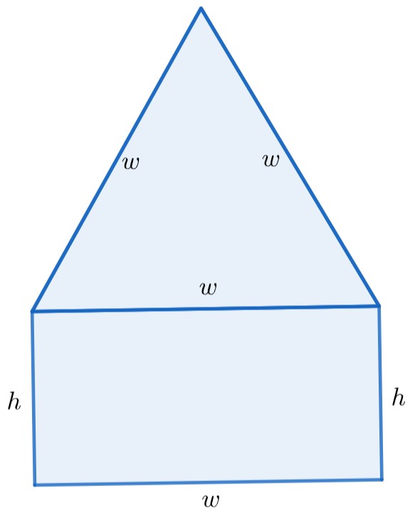
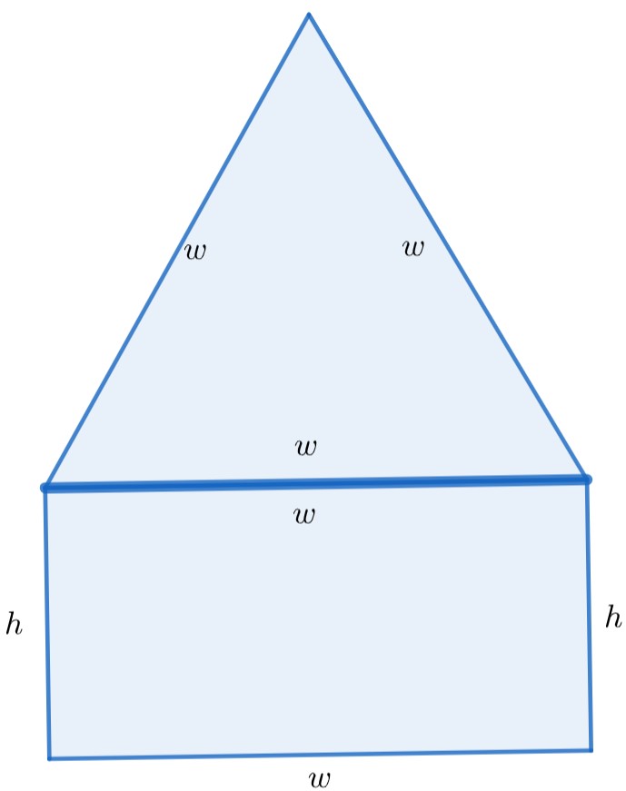
We're going to build a window in the shape of a rectangle topped by an equilateral triangle. We want to make a window which lets in the most light -- that is, with the greatest possible area. In order to build the window, we have to use wood trim. We have 16 feet of wood trim to build the window with.

Such a window has two dimensions: the width $w$ and the height $h$ of the rectangle. The rectangular portion has area $wh$ and the triangular portion has area $\frac{1}{2}w^2\text{.}$ So the total area is

\begin{equation*} A(w,h)=wh+\frac{1}{2}w^2\ . \end{equation*}

We also need to record the fact that our supplies are limited. A little geometry shows that to build the window requires two pieces of trim with length $h$ and four of length $w\text{.}$

Figure 9.2. A window made from a rectangle and a triangle.

Technically we don't have to use all the trim, but if we had some left over, we could have used it to build a bigger window. So let's assume we use all 16 feet; that is, we assume

\begin{equation*} 16=2h+4w\ . \end{equation*}

We can solve this equation for either $w$ or $h\text{.}$ Let's solve for $h\text{:}$

\begin{equation*} h=8-2w \end{equation*}

and substitute that into the formula for area:

\begin{equation*} A(w,h(w))=w(8-2w)+\frac{1}{2}w^2 \end{equation*}

Now we've got a function which we can optimize. We want to have a sensible result, so we know that $w$ can't be less than 0, and can be at most 4. So we want to optimize on the interval $\left[0,4\right]\text{.}$

Differentiating, we get $\frac{dA}{dw}=8-3w\text{.}$ So there is a single critical point at $w=\frac{8}{3}\text{.}$ We have

\begin{gather*} A(0,h(0))=0\\ A(4,h(4))=A(4,0)=\frac{1}{2}4^2=8\\ A\left(\frac{8}{3},h(\frac{8}{3})\right)=A\left(\frac{8}{3},\frac{8}{3}\right)=\left(\frac{8}{3}\right)^2+\frac{1}{2}\left(\frac{8}{3}\right)^2=\frac{32}{3} \end{gather*}

Since $\frac{32}{3}$ is greater than either 0 or 8, we see that the maximal area occurs when we choose width and height both equal to $\frac{8}{3}\text{.}$

This example shows a few things. First, notice that many optimization problems come equipped with a constraint. Here that was the fact that we only had so much trim. If you think about it, constrained optimization is the kind you usually deal with -- our world is full of scarcity.

Second, we can interpret each of the values we compared in the context of the problem. At $w=0\text{,}$ the window has width zero. At $w=4\text{,}$ $h=0$ so we only have a triangular section of window. $w=\frac{8}{3}$ is somewhere in between.

Third, the optimal dimensions happened to be equal to one another. This is typical -- optimizers are often symmetric (in this case, the symmetry is that $w$ and $h$ are the same.

Here are some other geometric optimization problems.

Checkpoint 111.

Given a total length of 10 meters of rope, what’s the greatest area we can enclose in a rectangle? Answer to three decimal places.

Using the same length of rope, what base length should we use to obtain the greatest area in an isoscees triangle? Answer to three decimal places.

Answer. 1

$6.25$

Answer. 2

$2.287$

Figure 9.3. Windows made from a rectangle and a triangle.

Checkpoint 112.

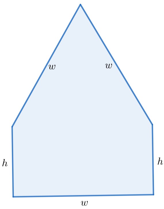
In the window example, let’s say we remove the “middle” piece of trim (which had length $w$). First, a gut check: does this increase or decrease the optimal area?

increase
decrease

What if we double up the middle trim? Does this increase or decrease the optimal area?

increase
decrease

Now verify your intuition by computing the optimal area in each scenario.

area with no crossbar:

area with double crossbar:

$\text{increase}$

$\text{decrease}$

$16$

$8$

Subsection 9.2 Optimization in economics and business

Let's think about production. A standard model, called the Cobb-Douglas production function, says that the productivity of a firm is proportional to both a power of the labor inputs $L$ and a power of the capital inputs $K\text{;}$ and that the powers add to 1. That is,

\begin{equation*} P=kK^\alpha L^\beta \end{equation*}

where k is the constant of proportionality and $\alpha+\beta=1\text{.}$ We may as well write $\beta=1-\alpha\text{,}$ so that our formula reads

\begin{equation*} P=kK^\alpha L^{1-\alpha}\ . \end{equation*}

Clearly, if we could increase $K$ and $L$ without constraint, we could increase the firm's output arbitrarily. But we have to operate subject to a budget. Spending more on labor means we have less to spend on capital, and vice versa. We model this by

\begin{equation*} B=K+L \end{equation*}

that is, the total budget is the sum of the captial costs and the labor costs.

A natural question to ask is: given a budget, how do we maximize output?

Just as with the window example, we manipulate our constraint to express one variable in terms of the other: $L=B-K\text{.}$ Then we substitute this into the objective function:

\begin{equation*} P(K,L(K))=k K^\alpha (B-K)^{1-\alpha}\ . \end{equation*}

That's a function we can optimize, on the interval $[0,B]\text{.}$

Checkpoint 113.

Let’s say $\alpha=\frac{1}{3}$ and $B=1000\text{.}$ What’s the optimal level of capital investment? Answer to the nearest cent.

Answer.

$\frac{1000}{3}$

Checkpoint 114.

Now solve symbolically.

If $\alpha=\frac{1}{3}\text{,}$ express the optimal capital investment in terms of the total budget $B\text{.}$

If $\alpha=\frac{1}{n}\text{,}$ express the optimal capital investment in terms of $n$ and the total budget $B\text{.}$

Answer. 1

$\frac{B}{3}$

Answer. 2

$\frac{B}{n}$

maximizing profit.

Consider the problem of a firm producing and selling a single good (say, pairs of sneakers). The goal of the firm is to make the most money possible.

Before we get into a precise model, let's set the ground rules.

production level: We'll call the number of pairs of sneakers we produce $t\text{.}$
production costs: We'll write $C(t)$ for the total cost of producing $t$ pairs of sneakers. $C(t)$ is an increasing function.
markets clear: We'll assume that we sell every pair of sneakers we make.
revenue: We'll write $R(t)$ for the total revenue that selling $t$ pairs of sneakers brings in. $R(t)$ is also an increasing function.
profit: The profit we make is $P(t)=R(t)-C(t)\text{.}$ Our goal is to maximize $P(t)\text{.}$

In finance and economics, the adjective marginal is used to denote a derivative. So we say marginal revenue to mean $R'(t)$ and marginal costs to mean $C'(t)\text{.}$

Checkpoint 115.

Based on the asumptions stated above, marginal revenue is

sometimes positive
sometimes negative
always positive
always negative

and marginal costs are

sometimes positive
sometimes negative
always positive
always negative

Answer. 1

$\text{always positive}$

Answer. 2

$\text{always positive}$

This use of the word $marginal$ comes from the fact that, using the tangent line approximation to $C(t)\text{,}$

\begin{align*} C(t+1)&\sim C(t)+C'(t)\left((t+1)-t\right)\\ C(t+1)&\sim C(t)+C'(t) \end{align*}

In other words, $C'(t)$ is approximately the additional cost added by the additional pair of sneakers that took us from production level $t$ to production level $t+1\text{.}$

In fact, thinking about derivatives this way can be very useful to understanding the situation of maximizing profit.

Checkpoint 116.

Put yourself in the shoes of a firm manager who gets to decide production levels.

If marginal costs (i.e. cost of producing the next pair of sneakers) are greater than marginal revenues (i.e. revenue generated by the next pair of sneakers), we should

increase
decrease
maintain current level of

the production level.

If marginal costs (i.e. cost of producing the next pair of sneakers) are less than marginal revenues (i.e. revenue generated by the next pair of sneakers), we should

increase
decrease
maintain current level of

the production level.

Be prepared to explain your answer in business terms.

Answer. 1

$\text{increase}$

Answer. 2

$\text{increase}$

Formally, we're trying to optimize

\begin{equation*} P(t)=R(t)-C(t) \end{equation*}

so our first step ought to be differentiating:

\begin{equation*} P'(t)=R'(t)-C'(t)\ . \end{equation*}

We want to find critical points of $P\text{;}$ that is, we need to solve

\begin{align*} P'(t)&=0\\ R'(t)-C'(t)&=0\\ R'(t)&=C'(t) \end{align*}

That is, we're looking for the production level where marginal cost and marginal revenue are equal.

Checkpoint 117.

As the manager of the firm, it’s your job to occasionally explain your decisions to the firm’s owner (who is mathematically illiterate). The owner sees the phrase marginal profit is zero in your written report and becomes quite upset. “Zero profit?!” he screams.

Explain to the owner why seeking zero marginal profit is the correct business decision.

modeling revenue.

Because profit is the difference of revenue and costs, understand how to solve $P'(t)=0$ amounts to understanding the revenue function $R(t)$ and the cost function $C(t)\text{.}$

Revenue seems straightforward. If we produce and sell $t$ pairs of sneakers for a price of $p$ dollars per sneaker, then

\begin{equation*} R(t)=p\cdot t \end{equation*}

But! the more sneakers we produce and sell, the less unique an individual wearing those sneakers is. The more sneakers we produce and sell, the fewer people go unshod. That tends to drive the price down. So the price $p$ isn't a constant; it's a function $p(t)$ of the number of pairs of sneakers we've sold.

Let's say that we've done some market research, and we've found that the market price of a pair of sneakers seems to obey

\begin{equation*} p(t)=300-.05t\text{.} \end{equation*}

Checkpoint 118.

In the formula $p(t)=300-.05t\text{,}$ what are the units of each of the following?

300:
- pairs of sneakers
- dollars
- pairs of sneaker per dollar
- dollars per pair of sneakers
- something else
t:
- pairs of sneakers
- dollars
- pairs of sneaker per dollar
- dollars per pair of sneakers
- something else
.05:
- pairs of sneakers
- dollars
- pairs of sneaker per dollar
- dollars per pair of sneakers
- something else

If you said “something else”, find the units.

Interpret what each of these numbers means in terms of the market price for sneakers.

Answer. 1

$\text{dollars per pair of sneakers}$

Answer. 2

$\text{pairs of sneakers}$

Answer. 3

$\text{something else}$

Notice that our model predicts that for high enough levels of production, $p(t)$ is negative. That is, if we completely saturate the market, we'd have to start paying people to take our sneakers (instead of them paying us). Is this prediction reasonable?

Checkpoint 119.

Write a formula for $R(t)$ if $p(t)=300-.05t\text{.}$

At what production level does maximum revenue occur?

Answer. 1

$\left(300-0.05t\right)t$

Answer. 2

$3000$

modeling costs.

What about costs? A standard model of costs is linear:

\begin{equation*} C(t)=C_0+mt \end{equation*}

where $C_0$ is called the fixed cost and represents the costs we have to spend no matter what: capital outlay for the factory, bribes for local politicans, etc.; and $m$ is the marginal cost (materials and labor to produce a single pair of sneakers).

Checkpoint 120.

I’ve used the phrase marginal cost in two different ways. Why are those two ways the same when the cost function looks like

\begin{equation*} C(t)=C_0+mt\ \ ? \end{equation*}

Let's say we build a factory for $10,000 and our marginal cost is $2 per pair of sneakers. Then we have

\begin{equation*} C(t)=10000+2t \end{equation*}

and

\begin{equation*} P(t)=t\cdot(300-.05t)-(10000+2t)\ \ . \end{equation*}

How do we acheive the maximum profit? When

\begin{equation*} 0=P'(t)=302-.1t \end{equation*}

which is $t=3020\text{.}$ The profit we actually make at that production level is $P(3020)=446,020\text{.}$ Not too bad.

Checkpoint 121.

What’s the production level which achieves maximum profit if our sneakers debut at $400 and market saturation reduces the price $0.50 per pair of sneakers in the market?

What is that maximum profit?

Answer. 1

$402$

Answer. 2

$70802$

But costs are not always linear. We say that a cost function obeys economies of scale if the marginal cost gets smaller as we increase the production level. For example, a worker producing their first pair of sneakers might take a lot of time, but by the time they get to their 30$^{th}$ pair of sneakers, the same worker can probably do so much more quickly (which means the labor cost for that pair of sneakers will be lower.

Checkpoint 122.

How do we encode economies of scale -- that is, decreasing marginal cost -- in calculus terms?

Just as we did with revenue, we can bootstrap our linear model for costs $C(t)=C_0+mt$ into a more model by replacing $m$ with $m(t)\text{.}$ If we think of our workers in the sneaker factory as gaining skill over time, then we could write something like

\begin{equation*} m(t)=1+\left(\frac{1}{2}\right)^{t/10} \end{equation*}

which is to say: the marginal cost starts at $2 per pair of sneakers, has a long-run limit of $1 per pair of sneakers, and every 10 pairs of sneakers produced moves the marginal cost halfway to the long-run limit.

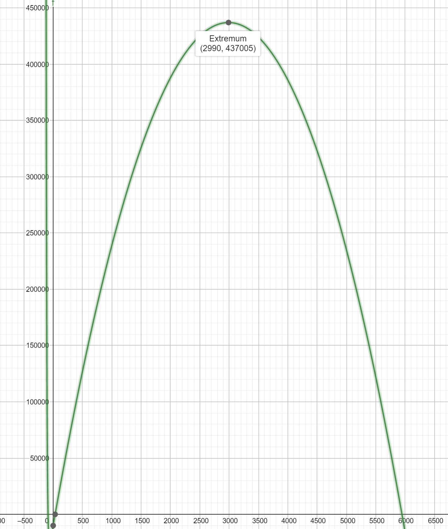
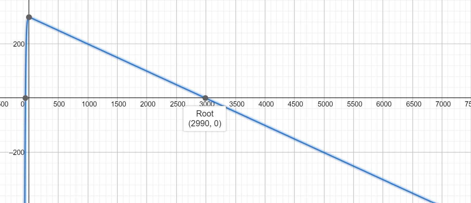
How do we achieve the maximum profit in this case? We have

\begin{align*} P(t)&=R(t)-C(t)\\ &=t\cdot(300-.05t)-\left(10000+\left(1+\left(\frac{1}{2}\right)^{t/10}\right)t\right) \end{align*}

which means that we need to solve

\begin{equation*} 0=P'(t)=299-.1t-\left(\frac{1}{2}\right)^{t/10}-\frac{1}{10}t\ln\left(\frac{1}{2}\right)\left(\frac{1}{2}\right)^{t/10}\ \ . \end{equation*}

Unfortunately there's not an algebraically clean solution to this equation, but a graphing utility says that $t=2990$ is very close.