Unit 3 Units, proportionality and mathematical modeling
Subsection 3.1 Physical units and formulas
One skill we'll need is writing formulas for functions given by verbal descriptions. Try this multiple choice question before going on.
Checkpoint 19.
Knowing that an inch is 2.54 centimeters, if \(f(x)\) is the mass of a bug \(x\) centimeters long, what function represents the mass of a bug \(x\) inches long?
\(\displaystyle 2.54 f(x)\)
\(\displaystyle \frac{f(x)}{2.54}\)
\(\displaystyle f\left(2.54 x\right)\)
\(\displaystyle f\left(\frac{x}{2.54}\right)\)
\(\text{Choice 3}\)
It helps to think about all such problems in units. Although inches are bigger than centimeters by a factor of \(2.54 \text{,}\) numbers giving lengths in inches are less than numbers giving lengths in centimeters by exactly this same factor. Writing this in units prevents you from making a mistake. The quantity 1 inch is the same as the quantity 2.54 centimeters, so their quotient in either order is the number 1 (unitless). We can multiply by 1 without changing something. Thus,
This shows that replacing \(x\) by \(2.54 x\) converts the measurement, hence is the correct answer.
Here are some more helpful facts about units.
- You can't add or subtract quantities unless they have the same units. That would be like adding apples and oranges!
- Multiplying (resp. dividing) quantities multiplies (resp. divides) the units.
- Taking a power raises the units to that power. For example, if \(x \) is in units of length, say centimeters, then \(3 x^2 \) will have units of area, in this case square centimeters. Most functions other than powers require unitless quantites for their input. For example, in a formula \(y = e^{***} \) the quantity *** must be unitless. The same is true of logarithms and trig functions: their arguments are always unitless.
- Units tell you how a quantity transforms under scale changes. For example a square inch is \(2.54^2 \) times as big as a square centimeter.
Checkpoint 20.
Suppose a pear growing on a tree doubles in length over the course of two weeks. By what factor does its volume increase?
\(8\)
Often what we can easily tell about a function is that it is proportional to some combination of other quantities, where the constant of proportionality may or may not be known, or may vary from one version of the problem to another. Constants of proportionality have units, which may be computed from the fact that both sides of an equation must have the same units.
Example 3.1.
If the monetization of a social networking app is proportional to the square of the number of subscribers (this representing perhaps the amount of messaging going on) then one might write \(M = k N^2 \) where \(M \) is monetization, \(N \) is number of subscribers and \(k \) is the constant of proportionality. You should always give units for such constants. They can be deduced from the units of everything else. The units of \(N \) are people and the units of \(M \) are dollars, so \(k \) is in dollars per square person. You can write the constant as \(k \; \frac{\$}{{\rm person}^2} \text{.}\)
To say \(A \) is inversely proportional to \(B \) means that \(A \) is proportional to \(1/B \text{.}\) If a quantity \(A \) is proportional to both quantities \(B \) and \(C \text{,}\) which can vary independently, then \(A \) must be proportional to \(B \cdot C \text{,}\) so \(A = k \; b \, C \) for some constant of proportionality, \(k \text{.}\)
Example 3.2.
If the expected profit on a home sale is proportional to the assessed value of the home and inversely proportional to the number of days it has been on the market, we could capture that relation as \(P = k V / T \) where \(P \) is profit in dollars, \(V \) is assessed price in dollars, \(T \) is number of days on the market, and \(k \) is a constant of proportionality.
Checkpoint 21.
What are the units of \(k\) in Example 3.2?
\(\text{day}\)
Warning 3.3.
Sometimes in mathematical modeling, an equation represents an empirical law, which is a rough fit to some function. For example, energy loss due to the nature of alternating current is said to be inversely proportional to the \(0.6 \) power of the frequency, but this is simply the best fit to data, not due to electromagnetic theory. In that case, units will not make sense. For example, if it is observed that the blood volume of small mammals is roughly proportional to the 2.65 power of the mammal's length, sensible units will not be assignable to the proportionality constant \(k \) in the formula \(BV = k L^{2.65} \text{.}\) In this case we just have to live with the fact that \(k \) has units involving fractional powers of length that won't make much sense outside of this context.
An important point when writing up your work: You don't just write \(M = k N^2 \) without stating the interpretations of the three variables. Also, there would not usually be a \(:= \) here, because you are not defining the function \(M(N) := k N^2 \) as much as you are saying that two observed quantities \(M \) and \(N \) vary together in a way that satisfies the equation \(M = k N^2 \text{.}\) There isn't a clear line here, but the style of the definition can be important in conveying to the reader what's going on.
Example 3.4.
The present value under constant discounting is given by \(V(t) = V_0 e^{-\alpha t} \) where \(V_0 \) is the initial value and \(\alpha \) is the discount rate. What are the units of \(\alpha \text{?}\) They have to be inverse time units because \(\alpha t \) must be unitless. A typical discount rate is 2% per year. You could say that as "\(0.02 \) inverse years." We hope that by the end of the semester, the notion of an inverse year is somewhat intuitive.
Checkpoint 22.
Write a formula expressing the statement that risk \(r\) (measured in percent) of viral infection in an enclosed space is proportional to the square of the number \(P\) of people and inversely proportional to the cube root of the volume \(V\) (measured in cubic feet) of the room. Use \(k\) for the constant of proportionality.
\(r=\)
What are the units of the constant of proportionality?
Often quantities are measured as proportions. For example, the proportional increase in sales is the change is sales divided by sales. In an equation: the proportional increase in \(S \) is \(\Delta S / S \text{.}\) Here, \(\Delta S \) is the difference between the new and old values of \(S \text{.}\) You can subtract because both have the same units (sales), so \(\Delta S \) has units of sales as well. That makes the proportional increase unitless. In fact proportions are always unitless.
Percentage increases are always unitless. In fact they are proportional increases multiplied by 100. Thus if the proportional increase is \(0.183 \text{,}\) the percentage increase is \(18.3\% \text{.}\) In this class we aren't going to be picky about proportion versus percentage. If you say thve percentage increase is \(0.183 \) or the proportional change is \(18.3\%\text{,}\) everyone will know exactly what you mean. But you may as well be precise.
Checkpoint 23.
The proportional increase in an animal’s weight during the first week of life is observed to be exponential in the percentage of a certain protein in the blood at birth. Do the units make sense?
yes
no
\(\text{yes}\)
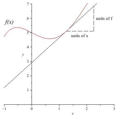
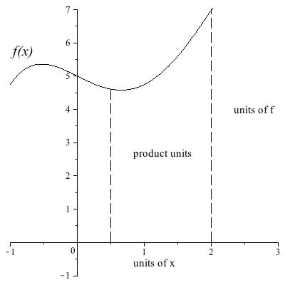
Units behave predictably under differentiation and integration as well. We will refer back to this when we define the relevant concepts, but you may as well see a preview now. The derivative \((d/dx) f \) has units of \(f \) divided by units of \(x \text{.}\) You can see this easily on the graph in Figure 3.5 because the derivative is a limit of rise over run, where rise has units of \(f \) and run has units of \(x \text{.}\) The integral \(\displaystyle\int f(x) \, dx \) has units of \(f \) times units of \(x \text{.}\) Again you can see it from a picture (Figure 3.6), because the integral is an area under a graph where the \(y\)-axis has units of \(f \) and the \(x\)-axis has units of, well, \(x \text{.}\)
Subsection 3.2 Modeling
Mathematical modeling means writing down mathematics corresponding to a given real-world (physical, chemical, biological) scenario, along with equations or other relations that could be expected to hold, at least approximately or under further assumptions.
Unpacking this, we see a number of features. First of all one must define mathematical objects in the model: variables, sets, functions, equations and so forth. Secondly, one must give interpretations of everything in the model. An interpretation tells what physical quantity is associated with each of the constants and variables and what relation is meant by each function. Real-world quantities include units, so this part always involves stating units. Thirdly, often one needs to add assumptions about the scenario. These say the circumstances under which would you expect the mathematics to be correct for the model. These assumptions are determined by the real world; they are not mathematical. Lastly, if there are questions given in the scenario, it is necessary to say what part of the mathematics answers the question(s). After this, what is left is a math problem: solve for the quantities that answer the questions.
In the following example, we have underlined parts of the modeling exercise that reflect the outline we have given, such as naming of variables, interpretation, units and hypotheses.
Example 3.7.
- Scenario
Galileo observes that objects falling a short time seem to fall a distance that was proportional to the square of the time and independent of the object: 4 feet for an object falling half a second, 9 feet after three quarters of a second, 16 feet after one second, and so forth. Galileo decides to measure the Tower of Pisa by dropping a stone from the top of the tower and measuring the time it takes for him to hear it hit the ground. Make a model for this and use it to estimate the elapsed time Galileo measure between dropping the stone and hearing the sound.
- Model
Let \(f(t)\) be the distance in feet that an object falls in \(t \) seconds, starting from rest. The wording of the scenario tells us that \(f(t) = c \, t^2\) where \(c \) has units of feet per seconds squared. This assumes we set \(t=0 \) at the time of release and measure distance from the point of release. We are asked to determine \(t \) such that \(f(t) = h\text{,}\) where \(h \) is the height of the Tower of Pisa. Equivalently, we need to find \(f^{-1} (h)\text{.}\) We assume that the model is accurate. What that means in this case is that we can ignore things such as air resistance and the time lag for the sound of impact to get back to Galileo's ear.
- Solution:
We look up the height of the Tower of Pisa to find that \(h = 186 \) feet. We solve for \(c \) given Galileo's data for small distances and find that \(c = 16 \) (for example: \(f(1/2) = c (1/2)^2 = 4 \) implies \(c=16\)). We can solve directly for \(16 t^2 = 186 \) or we can compute the inverse function to \(f \) yielding \(f^{-1} (x) = \sqrt{x/16} \) and substitute 186 for \(x \text{.}\) Either way we get \(t = \sqrt{186/16} \approx 3.40 \text{.}\) It may sound pedantic, but probably we should justify our choice of the positive square root by saying the whole experiment only covers time after the release, that is, \(t \geq 0 \text{.}\)
Were the physical assumptions warranted? Many objects would be slowed by air resistance over such a distance. Probably Galileo would have had to drop something like a rock in order for the fall not to have been significantly slowed. Looking up the speed of sound, it would take an extra \(1/4 \) second to register the sound. Probably Galileo could measure time to within greater accuracy that \(1/4 \) second, so this assumption is definitely shaky.
Checkpoint 24.
Example 3.7 states two physical assumptions -- that air resistance and time lag of sound are both negligible. But there are more physical assumptions built into the model than just those. Identify as many as you can.
For each physical assumption you identify, state whether it is reasonable or not.
Using units to interpret a model.
Sometimes we're given (or derive) a formula whose meaning isn't immediately clear; often the units can be our guide here. As an example, consider the body mass index (BMI), which medical researchers and doctors frequently use as a measure of obesity. BMI was invented by Adolphe Quetelet, a Belgian statistician, in the mid-1800s; it's still used today. (Think of how few medical tools from that period are still in use. . .)
A patient's BMI is computed by the following formula:
If we measure mass in kilograms and height in meters, the units of BMI are \(kg/m^2\text{.}\) That doesn't seem very revelatory.
But now consider: for objects of uniform density (which humans aren't, but close enough), we have
Substituting, we get
Now, broadly speaking, most people have approximately the same density. So when we compare two patients' BMIs, we're really comparing the quantity
which has units \(m^3/m^2=m\text{.}\) That is, roughly speaking BMI measures a length! But the length of what?
Here's were we need another rough biological fact: most peoples' width is proportional to their height; that is,
for some constant of proportionality \(k\text{.}\) If we pretend that a person's shape is a rectangular prism, then the volume of this prism would be
Because width is proportional to height, that works out to approximately
so that the quantity \(\frac{\text{volume}}{(\text{height})^2}\) is really
That is to say, what BMI really measures is how deep -- perhaps better to say, how thick -- a person is.
Checkpoint 25.
In the discussion above, we made several biological assumptions in order to interpret BMI as a measure of “body thickness”. Identify each such assumption and critique it.
Then think about the effect your critique would have on the usefulness of BMI as a measure of obesity.
By way of example: one assumption is that all humans have approximately the same density. Bodybuilders tend to have more muscle than the average person, and muscle is denser than other soft tissues; so the density of a bodybuilder will be above average. Therefore, bodybuilders will have a higher BMI -- that is, they will appear to be more obese than they are when measured with BMI.
Subsection 3.3 Inverse functions
One method of solving the problem of Galileo's experiment involved an inverse function. Let's be explicit about the definitions involved. The inverse function of a function \(f \) is the function that answers the question,
What input do I need to get the given output?
In other words, if \(g \) is the inverse function of \(f \) then \(g(y) \) is whatever value \(x \) satisfies \(f(x) = y \text{.}\) If there is more than one answer to this, then \(f \) has no inverse function; however, you can usually restrict the domain so there is only one answer. If there is no answer, that's not a problem, it just means that \(y \) is not in the domain of \(g \text{.}\) This happens when \(y \) is not in the range of \(f \text{.}\) Thus, the domain of \(g \) is the range of \(f \text{.}\) Likewise, the range of \(g \) is any possible answer to the question above, therefore any \(x \) in the domain of \(f \text{.}\)
Checkpoint 26.
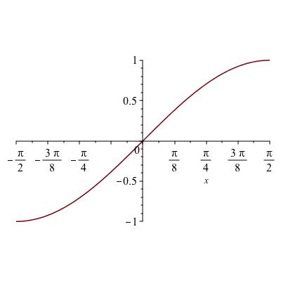
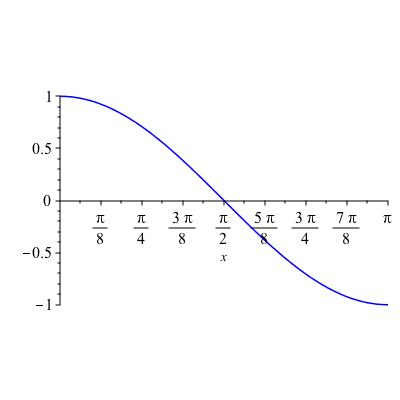
Let \(f(x) := \sin x\) on a domain of the form \([-L,L] \text{,}\) where \(L\) is some positive real number. What is the largest value of \(L\) such that \(f\) is one-to-one and therefore has an inverse?
\(1.5708\)
The usual notation for the inverse function to \(f \) is \(f^{-1} \text{.}\) This is terrible notation because it is the same as the notation for the \(-1 \) power of \(f \text{,}\) also known as \(1/f \text{.}\) We tried changing the inverse function notation to \(f^{\rm inv} \) for the purposes of this class, but then students were confused when they saw \(f^{-1} \text{.}\) We will stick with the terrible notation, and mention it when confusion might arise.
There is a standard way that the domain is restricted on trig functions so that the inverse function can be defined. For \(\sin \) and \(\tan \) it is \([-\pi/2 , \pi/2] \text{.}\) The function \(\cos \) when restricted to \([-\pi/2,\pi/2] \) is not one-to-one; the standard choice for \(\cos \) is \([0,\pi] \text{.}\) These are arbitrary conventions, but are probably built in to your calculator, so we had better adopt them. Also, along with \(\sin^{-1} \text{,}\) \(\cos^{-1} \) and \(\tan^{-1} \text{,}\) the conventional names \(\arcsin, \arccos \) and \(\arctan \) are also used.
Checkpoint 27.
Inverse functions occur naturally in mathematical modeling. For example, if \(f(t) \) represents how many miles you can walk in \(t \) hours, then \(f^{-1} (x) \) represents how many hours it takes you to walk \(x \) miles. Note that in this explanation, \(x \) is a bound variable; we could have used any other name, such as \(t \) again, only it helps readability if we use names such as \(t \) for time and \(x \) for distance.
Checkpoint 28.
Define \(f(x)\) to be the number of pounds you have to carry when planning a backpacking excursion for \(x\) days.
Consider the quantities \(f^{-1}(v)\text{,}\) \(f^{-1}(w)\text{,}\) and \(f^{-1}(v+w)\text{.}\)
What are the units of \(v\text{?}\)
What are the units of \(f^{-1}(v)\text{?}\)
Give an interpretation for \(f^{-1}(v)\)
Give interpretations for \(f^{-1} (v) + f^{-1} (w)\) and \(f^{-1} (v+w)\)
Between \(f^{-1} (v) + f^{-1} (w)\) and \(f^{-1} (v+w)\text{,}\) which do you think would be greater?
Remark 3.9.
The concept of an inverse function appears to be harder than most people realize. For example, a number of years ago, calculus students were given the problem to compute a formula for the inverse function to \(\sinh (x) \text{,}\) the hyperbolic sine function. This was already not easy: (only half the students got it) but then we asked them to find a number \(u \) such that \(\sinh (u) = 1 \text{.}\) Almost no one got it, despite that fact that this was supposed to be the easy part -- they just needed to plug in 1 to their inverse sinh function! By definition, \(\sinh^{-1} (1) \) is a number \(u \) such that \(\sinh (u) = 1 \text{.}\) The moral of the story is, don't lose sight of the meaning of an inverse function when doing computations with them.
How does the graph of an inverse function relate to the graph of a function? The roles of \(x \) and \(y \) have switched. When the first and second coordinate of an ordered pair are switched, the point reflects across the diagonal line \(y=x \text{.}\) Thus, the graph of the inverse function is the original graph (on the appropriate domain) reflected across the diagonal.
Logarithm Cheat Sheet.
The inverse function to \(f(x):=e^x\) is called the nautral logarithm \(\ln\text{.}\) All that means is: the equations
and
mean exactly the same thing. Logarithms look scary, but all you have to remember is: when you see a logarithm on one side, just convert the whole equation to exponentials.
It may be useful to have some approximate values of \(\ln\) in mind so that the function seems less mysterious. The following values are accurate to about 1%:
Checkpoint 29.
In the list of approximations above, convert each statement about logarithms into the corresponding statement about exponentials, and vice versa.
In case you need them, here are some other useful quantities to within 1%:
Also useful sometimes: \(\sqrt{3} = 1.732\ldots \) and \(\sqrt{5} = 2.236\ldots \) both to within about \(0.003\% \text{.}\)
Checkpoint 30.
Squares and Powers of 2 Cheat Sheet.
If you know the powers of 2 you can do the same thing with \(\log_2 \) that you can do with \(\log_{10} \text{.}\) It will be helpful for you be at least somewhat familiar with them -- for example, to recognize them on sight. You should also recognize the first twenty squares:
No kidding, when you come across one of these numbers under a radical, you know immediately it can be factored out.
Here are the powers of 2.
Subsection 3.4 Exponential and logarithmic relationships
Taking a break from heady stuff, let's do some quick computations with logs.
The log cheatsheet is there to encourage you to use logs for quick computations. The squares and powers of two are just for fun (OK it was written by geeks). We're going to take a quick break from concepts to get the hang of computing with logs.
Example 3.10.
What is the probability of getting all sixes when rolling 10 six-sided dice? It's 1 in \(6^{10} \) but how big is that? If we use base-10 logs, we see that
So the number we're looking for is approximately \(10^{7.8} \) which is \(10^7 \times 10^{0.8} \) or \(10,000,000 \) times a shade over \(10^{.78} \text{,}\) this latter quantity being very close to 6 according to the one-digit logs you computed. So we're looking at a little over sixty million to one odds against.
Checkpoint 31.
Roughly how big is \(5^{11} \text{?}\) Just one significant digit is fine.
\(8.1\times 10^{7}\)
These are not just random examples, it is always the best way to get a quick idea of the size of a large power. When the base is 10 we already know how many digits is has, but when the base is something else, we quickly compute \(\log_{10} (b^a) = a \cdot \log_{10} (b) \text{.}\)
Example 3.11.
Why is the value \(\ln (10) \approx 2.3 \) on your log cheatsheet so important? It converts back and forth between natural and base-10 logs. Remember, \(\log_{10} x = \ln x / \ln 10 \text{.}\) Thus the constant \(\ln 10 \) is an important conversion constant that just happens to be closer than it looks (the actual value is \(2.302\ldots\)). So for example,
Checkpoint 32.
A certain astronomical computation yields the number \(e^{24} \text{.}\) How many digits will this be? (Meaning, how many digits before the decimal point.)
\(11\)
Recall in the definition of \(e \text{,}\) the slope of the graph \(e^x \) at \((0,1) \) is 1, therefore the tangent line approximation is
This approximation is very good when \(x \lt 0.1 \text{.}\) Converting to logs gives the version
which the following example illustrates the utility of.
Example 3.12.
Suppose, your company grows in value by 6% each year for 20 years. By what factor \(C \) does the value increase over this time? The answer is \(1.06^{20} \text{,}\) but about how big is that? For a quick answer, take logs. Using the fact that \(\ln 1.06 \approx 0.06 \) (that's the logarithmic version of our estimate, with \(x=.06\)), we see that \(\ln C = \ln (1.06^{20}) \approx 20 \times 0.06 = 1.2 \text{.}\) We'd rather have this in base ten, so we compute
maybe a little bigger like \(0.52 \) or so. Looking at the log cheatsheet shows this means \(C \) should be between 3 and 4, somewhat closer to 3. In fact to two significant figures, the growth factor is 3.2.
Checkpoint 33.
Historical economists look at real (inflation-adjusted) growth rates over periods of a century or more. If the real annual growth rate averages 2%, what should be the growth factor over the century and a half from 1870 to 2020? Use the method given in Example 3.12 and answer with a whole number.
Now use a calculator to compute the exact answer, accurate to one decimal place.
The multiplicative frame.
If you ask someone to state a relationship between the numbers 20 and 30, the most common answer is that 30 is ten more than 20. A more fundamental answer is that 30 is 50% more, or equivalently that 30 is three halves of 20. The section on proportionality is designed to emphasize multipicative thinking over additive thinking. Additive thinking is more common only because we find it computationally easier to add than to multiply. Saying that multiplicative thinking is more fundamental is not a precise mathematical statement, so there's no way to prove it. One reason to believe it is that mulitplicative statements remain the same no matter what units you use (as long as the 30 and the 20 are in the same units).
Checkpoint 34.
A small city has 40,000 households. To organize an emergency response system, the city wants to organize groups of households on a scale “halfway between the individual household and entire city scale.” What size of groups of households best fulfills this?
Exponentials and logarithms are built to express multiplicative facts. In fact the additive laws of exponentiation and logarithms basically convert multiplicative facts to additive facts, thereby converting the more fundamental fact to the type you can compute more easily.
Much of what you learn on topic of exponential and logarithmic relationships involves questions such as:
If you observe that \(\ln x \) has increased by about \(0.7 \text{,}\) what does this mean about the increase that has occurred in \(x \text{?}\)
A tip about setting up equations representing functional relationships: when a quantity has different values at different times such as "before" and "after", using one variable to represent both quantities can lead to mess and confusion. Better to use different names such as \(x_1 \) and \(x_2 \text{,}\) or \(x_{\rm init} \) and \(x_{\rm final} \text{,}\) or possibly \(x \) and \(x' \text{,}\) etc. Using this idea on the question above sets up an equation like this: \(\ln x_2 \approx \ln x_1 + 0.7 \text{.}\) From here, exponentiating leads to
So, if you observe \(\ln x \) increasing by about 0.7, you will know that \(x \) had approximately doubled. This is what it means that logarithms transfer multiplicative scales to additive ones. A multiplicative relation such as doubling transfers to an additive relation, namely addition of about 0.7.
Checkpoint 35.
When \(x\) triples, what happens to the base-ten log of \(x \text{?}\)
The base-10 log of \(x\) triples.
The base-10 log of \(x\) is cubed.
The base-10 log of \(x\) is divided by 3.
The base-10 log of \(x\) decreases by about .477.
The base-10 log of \(x\) decreases by about 1.099.
It depends on what \(x\) is.
What about the natural log of \(x \text{?}\)
The natural log of \(x\) triples.
The natural log of \(x\) is cubed.
The natural log of \(x\) is divided by 3.
The natural log of \(x\) decreases by about .477.
The base-10 log of \(x\) decreases by about 1.099.
It depends on what \(x\) is.
If \(\ln x\) has tripled, what has happened to \(x \text{?}\)
\(x\) has tripled.
\(x\) has been cubed.
\(x\) has been divided by 3.
\(x\) has decreased by about .477.
\(x\) has decreased by about 1.099.
It depends on what \(x\) is.
One more thing to keep in mind about logarithms and exponentials is that they do not scale with units. If we change the units of \(x \) from inches to centimeters, and if \(y = e^x \text{,}\) then in the new units \(y' = e^{2.54 x'} = y^{2.54} \text{.}\) The new exponential appears to be the old one to the 2.54 power. What does that even mean? It is a tipoff that \(x \) should not be exponentiated: anything other than a unitless constant is likely to be meaningless when exponentiated. The same is true for logarithms and trig functions.
If \(\log x \) increases at a constant additive rate, then \(x \) increases at a constant multiplicative rate. What does this mean?
If a quantity \(Q \) increases at a constant additive rate, it means that if you wait one unit of time, \(Q \) always increases by the same additive amount. In fact, between any two times \(s \) and \(t \) the increase will be \(c (t-s) \text{.}\)
Checkpoint 36.
If \(Q\) increases at a constant additive rate, what are the units of \(c \text{?}\)
units of \(Q\)
units of \(Q\) divided by units of \(t\)
units of \(t\)
units of \(Q\) times units of \(t\)
\(c\) is unitless
\(\text{Choice 2}\)
If a quantity \(Q \) increases at a constant multiplicative rate, it means waiting one unit of time always multiples \(Q \) by the same amount, and in general, between times \(s \) and \(t \text{,}\) the factor by which \(Q \) increases will be \(c^{t-s} \) where \(c \) is the factor by which \(Q \) increases in one unit of time.
Checkpoint 37.
If \(Q\) increases at a constant multiplicative rate, what are the units of \(c \text{?}\)
units of \(Q\)
units of \(Q\) divided by units of \(t\)
units of \(t\)
units of \(Q\) times units of \(t\)
\(c\) is unitless
\(\text{Choice 5}\)
To get back to the question of what it means about logs relating additive to multiplicative growth, if \(\log x = a + bt \) (constant additive growth over time) then \(x = e^{a + bt} = e^a e^{bt} = A B^t \) where \(A = e^a \) and \(B = e^b \text{.}\) This is constant multiplicative growth.
Constant multiplicative growth rates occur in a lot of applications. This is also called exponential growth because the formula for a quantity growing multiplicatively is \(A e^{bt} \) (also \(e^{a+bt} \) or \(A B^t\)). When \(b \lt 0 \text{,}\) it is called exponential decay or decrease.
Here are a few examples.
- Equilibrating temperatures
If an item is hotter or colder than its environment then the temperature difference between the object and its environment, as a function of time, decreases exponentially (here, in \(A e^{bt} \text{,}\) the coefficient \(b \) is negative).
- Accumulating money
At a fixed interest rate, money grows exponentially. So, unfortunately does debt (just put a minus sign on the money).
- Population
Populations tend to grow this way (again unfortunately, in most cases).
- Radioactive substances
decay exponentially.
- DNA
The portion of DNA remaining unmutated decays exponentially.
- Present value analysis
If there is a fixed discount rate, there is exponential decrease of the present value for revenue at future times.
- Time series data
Not always, but often, the correlation decays exponentially.
If we get to assume a nice clean exponential model, and can observe at more than one time point, then exponential growth/decay models are nearly as easy to solve as linear growth models (a highlight of eighth grade math). You should learn this both conceptually and as a mindless skill. In Math 104, this is taught as an elementary example of differential equations. We'll get to those next semester, but really this kind of growth/decay model is far more fundamental and should be discussed now. Here's an example of how the computation goes.
Example 3.13.
A viral infection is spreading exponentially through the community. On the first day that the outbreak had a name, there were 25 infections. A week later there were 40 infections. How many infections will there be in another two weeks? When will the number of infections reach 200,000, which is the size of the entire local population?
- Solution #1 (plug in logs)
-
Let \(N(t) \) denote the number of infections after \(t \) weeks. Our model is \(N(t) = A e^{bt} \text{.}\) The given information is that plugging in \(t=0 \) and \(t=1 \) give \(N = 25 \) and \(N=40 \) respectively. Because \(e^0 = 1 \text{,}\) we have \(25 = A \text{,}\) while \(40 = A e^b \text{.}\) This gives \(e^b = 40/25 = 8/5 \text{,}\) hence \(b = \ln (8/5) \text{.}\) In another two weeks we will have \(t=3 \text{,}\) so
\begin{equation*} N(3) = 25 e^{3 \ln (8/5)} \, . \end{equation*}When \(N=200,000 \) we have \(25 e^{t \log (8/5)} = 200,000 \) hence
\begin{equation*} e^{t \ln (8/5)} = \frac{200,000}{25} = 8,000 \text{ hence } t = \frac{\ln 8000}{\ln (8/5)} \approx 19.12\, . \end{equation*} - Solution #2 (growth factor)
-
If we use the growth factor \(B \) in the equation \(A B^t \) instead of the exponential constant \(b \) in \(A e^{bt} \) we may get away without logs. In a week the increase was from 25 to 40, a factor of \(8/5 \) so clearly \(B = 8/5 \text{.}\) Thus \(N = 25 (8/5)^t \text{.}\) In three weeks we have \(N(3) = 25 (8/5)^3 = 512/5 = 102.5 \text{.}\) Evidently the expression \(25 e^{3 \ln (8/5)} \) can be simplified! The time needed to get to 200,000, a growth factor of 8000, is \(t \) such that \((8/5)^t = 8000 \text{.}\) This is, by definition \(\log_{8/5} 8000 \text{,}\) which is equal to \(\log_b 8000 / \log_b (8/5) \) for any base \(b\text{.}\) If we pick \(b=10\text{,}\) we get
\begin{equation*} t = \frac{\log 8000}{\log (8/5)}\approx 19.12 \, . \end{equation*}
Notice that that the answer given by plugging in logs is a special case of the growth factor approach, using base \(e \text{.}\) But the ratio of two logs is the same in any base! In Solution 2, we can use what we know about \(\log_{10}\) to compute
Having converted everything to logs of single digits, we can approximate by
So it should take between nineteen and twenty weeks to saturate the city. That's close enough to the more precise answer that we obtained from a calculator.
Checkpoint 38.
Is exponential growth a more realistic model when a small portion of the population is infected or when a large portion is infected?
The following exercise is a little more involved than the usual self-check exercise. It will be more readily solved if you realize that computations in the exponential model for equilibrating temperatures work better if you keep track of the temperature difference between substance and the environment rather than the temperature of the substance on its own.
Checkpoint 39.
Room temperature is \(70^\circ \) F. The temperature of a cup of coffee is \(205^\circ \) F (it's from McDonald's, where they make strikingly hot coffee). In 10 minutes it's a barely sippable \(160^\circ \) F. About how many minutes after purchase is a cup of coffee gulpable (\(130^\circ \) F)? Body temperature (\(98.6^\circ\))? Approximate answers are fine, but please don't forget to name your variables, give units, etc.