Unit 11 Integrals
Subsection 11.1 Area
Integrals compute many things, the most fundamental of these being area. The definition of area is more subtle than one might think. Most people's understanding of area is based on a physical concept of how much two-dimensional space is taken up. For example, if you have to paint an irregular flat shape, how much paint does it take?
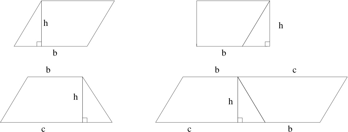
Looking back at the treatment of area in the pre-college math curriculum, you can see the steps toward a mathematical definition. First, for rectangles with integer sides \(a\) and \(b\text{,}\) you can count the number of \(1 \times 1\) squares needed to make the rectangle, leading to the area formula \(A = a \times b\text{.}\) From the physical point of view this is a formula, but from the mathematical point of view it is a definition, extended later to non-integer side lengths. Areas of triangles are not studied until much later. For right triangles with sides \(a\) and \(b\) and hypotenuse \(c\text{,}\) the area is shown to be equal \(ab/2\) by showing that two of these fit together to make an \(a \times b\) rectangle. This invokes a new principle: areas of congruent figures are equal. To compute the area of a parallelogram or trapezoid, the dissection principle is invoked: cutting up and rearranging the pieces of a figure preserves the area. These principles, all of which make intuitive and physical sense, are illustrated in Figure 11.1.
Checkpoint 136.
Write a sentence for each of the two rows explaining how it establishes an area formula. What is being asserted to have the same area as what, why is this true, and what is the conclusion?
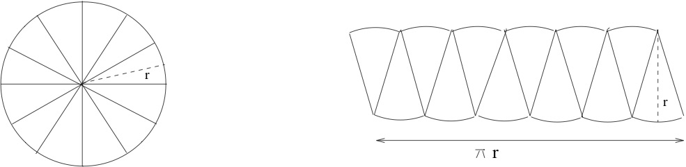
The area of a circle is introduced, usually without much explanation. Do you know why the area of a circle of radius \(r\) is equal to \(\pi r^2\text{?}\) One common explanation is that areas of similar figures are related by a scaling principle. Recalling that area has units of squared length, it makes sense that scaling a figure by \(\lambda\) should scale the area by \(\lambda^2\text{.}\) All circles are similar; if follows that the area of a circle should be \(K r^2\) for some constant \(K\text{.}\) We can name this constant \(\pi\) but that leaves a nagging question unanswered. Scaling also shows that the circumference of a circle should be proportional to the radius, therefore \(C = K' r\) for some other constant \(K'\text{.}\) This turns out to be \(2 \pi\text{.}\) But why should \(K'\) be double \(K\text{?}\) An argument involving dissections and limits is shown in Figure 11.2.
Checkpoint 137.
In Figure 11.2 the measure \(\pi r\) on the right refers to the total curved length of the bottom.
We have not defined limits of shapes, but intuitively, what is the limiting shape on the right?
What are its dimensions? by
Once limits are brought into the discussion, there is a way to define areas of much more general shapes. The idea is this: put as many non-overlapping squares of some small side length \(\varepsilon\) as you can inside the shape. These cover an area less than the area of the shape, but if \(\varepsilon\) is small, it seems credible that the area is getting close to the area of the shape. If the limit as \(\varepsilon \to 0^+\) exists, this should be the area of the shape. Similarly, you could completely cover the shape with squares of side \(\varepsilon\) if you are willing to cover a slightly too big region. When \(\varepsilon\) is small, you don't cover too much extra area. The limit as \(\varepsilon \to 0^+\) should also be the area of the shape. To make a long story short (you can hear the full story in Math 360), there are many shapes for which it is possible to prove that these two limits exist and are equal. For these shapes we can define area to be this common limiting value. This mathematical definition captures our existing physical intuition and is also consistent with the principles we already adpoted: congrunce, scaling and dissection.
Subsection 11.2 Riemann sums and the definite integral
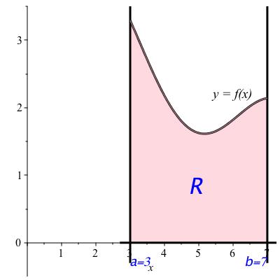
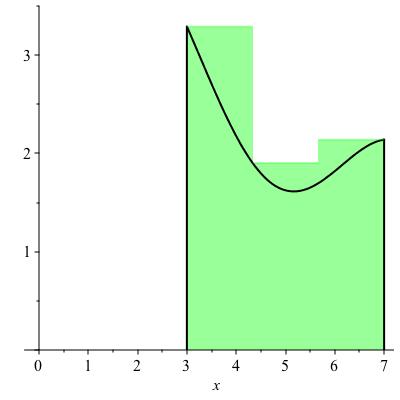
With this build up, we will give a mathematical definition for the area for a certain restricted class of shapes. These are rectangular on three sides but whose top is described by a continuous function. More precisely, let \(a \lt b\) be real numbers and let \(f\) be positive and continuous on the closed interval \([a,b]\text{.}\) We will define the area of the region \(R\) bounded on the left by the vertical line \(x=a\text{,}\) on the right by the vertical line \(x=b\text{,}\) on the bottom by the \(x\)-axis (the line \(y=0\)), and on the top by the graph of \(f\) (the curve \(y = f(x)\)). This region is shown in Figure 11.3.
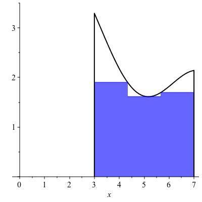
We now define the lower and upper Riemann sums with \(n\) rectangles for a function \(f\) on an interval \([a,b]\text{.}\) If you prefer a picture, refer to Figure 11.4.
Checkpoint 138.
In Figure 11.4, what value of \(n\) was used?
\(3\)
Definition 11.5.
Let \(f\) be a nonnegative continuous function on an interval \([a,b]\) and let \(n\) be a positive integer. Let \(I_1, \ldots , I_n\) denote the intervals you get when you divide \([a,b]\) into \(n\) equally sized intervals. For each interval \(I_k\text{,}\) let \(y_k\) be the minimum value of \(f\) on \(I_k\) and let \(R_k\) be the rectangle with base \(I_k\) on the \(x\)-axis and height \(y_k\text{.}\) The lower Riemann sum for \(f\) on \([a,b]\) with \(n\) rectangles is the sum of the areas of the rectangles \(R_k\text{,}\) for \(1 \leq k \leq n\text{.}\) The upper Riemman sum is defined similarly, with the maximum value instead of the minimum value on each interval.
Checkpoint 139.
Example 11.6.
We are not given precise values for the function \(f\) in Figure 11.4, but we can estimate from the graph. The rectangles each have width \(4/3\text{.}\) The respective heights for the lower Riemann sum appear to be roughly \(1.9, 1.6\) and \(1.7\text{,}\) making the lower Riemann sum equal to \((4/3) 1.9 + (4/3) 1.6 + (4/3) 1.7 = (4/3) 5.2 \approx 6.93\text{.}\) The upper Rieman sum is computed from rectangles with approximate heights \(3.3, 1.9\) and \(2.15\text{,}\) leading to a total area of \((4/3) 7.35 = 9.8\text{.}\)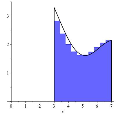
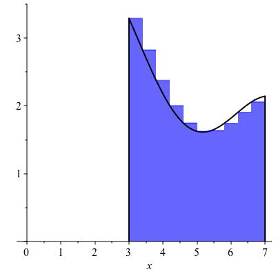
The left Riemann sums and right Riemann sums are defined similarly, except that instead of using the minimum or maximum values of the function on each sub-interval the left Riemann sums uses the value at the left endpoint of each interval \(I_k\text{,}\) while the right Riemann sum uses the value at the right endpoint of each sub-interval \(I_k\text{.}\) Examples are shown in Figure 11.7.
Checkpoint 140.
Which of the two images in Figure 11.7 is the left Riemann sum?
the graph on the left is a left Riemann sum
the graph on the right is a left Riemann sum
\(\text{the graph ... Riemann sum}\)
The upper and lower Riemann sums give upper and lower bounds on the area of the figure. The left and right Riemann sums are neither upper nor lower bounds for the area, but they are sandwiched in between the lower and upper Riemann sums, so they also converge to the area. They are useful because always choosing the left endpoint (or always choosing the right endpoint) leads to a simpler formula.
Checkpoint 141.
Write a summation formula for the left Riemann sum for \(f\) on \([a,b]\) with 10 rectangles. It should have 10 terms and look like this:
\(\displaystyle\sum_{n=1}^{10}\)
\(\frac{f\!\left(a+\frac{\left(n-1\right)\!\left(b-a\right)}{10}\right)\!\left(b-a\right)}{10}\)
The values of the lower and upper Riemann sums in Figure 11.4 are approximately \(6.9\) and \(9.8\text{.}\) These are not very close to each other, leaving considerable uncertainty about the true area. Replacing by the left (say) Riemann sums, we can program the sum into a computing device and compute for much greater values of \(n\text{.}\) If we increase \(n\) from 3 to 10, as in Figure 11.7, we find the Riemann sums come out to approximately 8.48 and 8.02 -- somewhat better. These are not necessarily bounds: the true value could be greater than both, or less than both, or in between. Replacing \(n\) by 50 gives 8.28. This is again not a bound, however the following theorem guarantees that as \(n \to \infty\text{,}\) this will converge to the area.
Theorem 11.8.
The upper Riemann sums for any continuous function \(f\) on any closed interval \([a,b]\) converge as \(n \to \infty\text{.}\) The lower Riemann sums converge to the same value. It follows that you can let \(y_k = f(x_k)\) for any\(x_k \in I_k\) and the sums of rectangle areas will still converge to this common limit.Definition 11.9.
The common limit in Theorem 11.8 is called the definite integral of \(f\) from \(a\) to \(b\) and is denoted \(\displaystyle\int_a^b f(x) \, dx\text{.}\)
Checkpoint 142.
Let \(f\) be the constant function \(c\text{.}\) How far apart are the lower and upper Riemann sums for \(\displaystyle\int_3^9 c \, dx\) (pick any value of \(n\))?
What does that tell you about the definite integral \(\displaystyle\int_a^b c \, dx\text{?}\)
Remark 11.10.
The variable \(x\) is a bound variable; the notation \(\displaystyle\int_a^b f(u) \, du\) would represent the same thing. Also, as in the notation for derivatives, you shouldn't try to interpret what the symbol \(du\) means on its own. It evokes the width of an infinitesimal rectangle, but you can't always count on it to behave nicely in equations.Checkpoint 143.
From this construction and theorem, you can deduce some identities for integrals.
Let’s say we know that \(\displaystyle\int_a^bf(x)\ dx=3\) and \(\displaystyle \int_b^c f(x)\ dx=5\text{.}\) Compute each of the following:
\(\displaystyle\int_a^b f(x) \, dx + \displaystyle\int_b^c f(x) \, dx=\)
\(\displaystyle\int_a^b 3 + 10 f(x) \, dx=\)
Subsection 11.3 Interpretations of the integral
Area is the most visually obvious interpretation but there are many others. If material (or charge, or mass, etc.) is spread out unevenly over an interval, the density at any point is the amount of material per length near that point. It has units of material divided by length. The total amount of material in the interval is gotten by summing how the amount of material over small intervals. When the interval is small enough, we can estimate the amount of material as \(f(x)\) times the length of the interval where \(x\) is any point in the interval. This is not exact because \(f\) generally will still vary over the interval, but not by much when \(x\) is small. The limit as the interval lengths go to zero will be \(\displaystyle\int_a^b f(x) \, dx\) and will represent the total material.
Example 11.11.
A 3-inch blade of grass is covered in mold. The amount of mold decreases up the blade because it is killed by sunlight. The density of mold per inch is \(1000 e^{-x/3}\) spores per inch at height \(x\) inches from the ground. The total number of spores on the blade of grass is given by \(\displaystyle\int_0^3 1000 e^{-x/3} \, dx\text{.}\)
Checkpoint 144.
Why did we use 0 and 3 for the limits of integration in Example 11.11?
Definition 11.12. average over an interval.
The average of a quantity varying over an interval \([a,b]\) according to a function \(f\) is defined to be \(\frac{1}{b-a} \displaystyle\int_a^b f(x) \, dx\text{.}\)
Example 11.13.
Suppose the temperature over a day is \(f(t)\) degrees Celsius \(t\) hours after midnight. The average temperature over the day is then \(\frac{1}{24} {\displaystyle\int_0^{24} f(t) \, dt}\text{.}\)
Checkpoint 145.
Suppose \(f(x)\) is some constant \(c\) on the interval \([a,b]\text{.}\) Intuitively, what is the average of \(f\) on \([a,b]\text{?}\) Compute the average value of \(f\) on \([a,b]\) directly from the definitions and check that it is what you expected.
An integral is a limit of a sum of rectangles' areas. The units are therefore the same units as the rectangles' areas. The rectangles live on a graph where the \(x\)-axis has units of the argument variable and the \(y\)-axis has units of the function. Therefore the rectangle units, hence the integral units, are units of the argument times units of the function. In the grass example, the function was density (spores per inch) and the argument was inches, therefore the integral had units of spores. It is a good thing that this agrees with our interpretation of the integral as the total number of spores. In the temperature example, \(f\) has units of temperature and \(t\) is in units of time, so the integral of \(f\) has units of temperature times time. This sounds like a strange unit but it's not unheard of. Severity of cold spells is measured, for example, in heating degree-days. The average is the integral divided by the time, so it is in units of temperature. Of course: the average temperature should be a temperature!
In physics there are countless things represented by integrals. One is the moment. Suppose mass is spread out along \([a,b]\) with density \(f\) (you know what that means now, right?). Integrate \(f\) and you get the total mass. If instead you compute \(\displaystyle\int_a^b x \, f(x) \, dx\) you get the moment of inertia, which tells you how much the weight counts when balancing (imagine a teeter-totter pivoting on the origin), or how much torque is needed to produce a given angular acceleration.
In probability theory, random quantities can be discrete or continuous. If the random quantity \(X\) is discrete it means that there is a sset of values \(x_1, x_2 , \ldots\) such that probabilities for \(X = x_k\) sum to 1. This could be a finite sum or the sum of an infinite sequence (you now know the definition of an infinite sum, right?). For continuous quantities, you need integrals. The probabilities for finding \(X\) to take various values are spread continuously over an interval (possibly an infinite interval such as the whole real line). There will be a probability density function \(f\) such that the probability of finding \(X\) in a given interval \([a,b]\) will be \(\displaystyle\int_a^b f(x) \, dx\text{.}\) We will say more about this in Unit 13, after we have defined integrals where one or both of the limits of integration can be infinite.
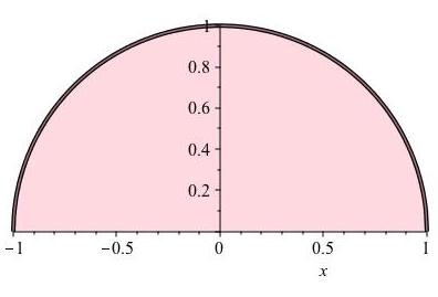
Going back to the area interpretation, you may ask what about more general shapes? It turns out you don't really need straight sides. The vertical walls on the left and right sides of the regions Figure 11.3 and Figure 11.4 can disappear. For example, letting \(f(x) = \sqrt{1-x^2}\) and \([a,b] = [-1,1]\) produces the upper half of a disk.
So far we have required \(f\) to be a nonnegative function. What if \(f\) is negative?
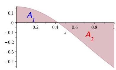
Let \(\Delta_k\) denote the width of \(I_k\text{.}\) The most useful definition turns out to be that the integral is still the limit of sums of the quantities \(\displaystyle\sum_k f(x_k) \cdot \Delta_k\) but we must interpret this as a new concept, called signed area rather than area. We won't worry too much about signed area; it just means we need to keep track of whether \(f\) is positive or negative before we know whether \(\displaystyle\int_a^b f(x) \, dx\) computes area or its negative. Figure 11.14 shows a function which is positive on \([0,0.42]\) and negative on the interval \([0.42,1]\text{.}\) The integral \(\displaystyle\int_0^1 f(x) \, dx\) will be slightly negative because it adds a positive area \(A_1\) to a negative signed area \(A_2\text{.}\)
Another useful definition along the same lines switches the upper and lower limits.
Definition 11.15.
If \(a < b\) then \(\displaystyle\int_b^a f(x) \, dx\) is defined to equal \(- \displaystyle\int_a^b f(x) \, dx\text{.}\)Suppose \(f\) and \(g\) are functions such that \(f \geq g\) on \([a,b]\text{.}\) One interpretation of \(\displaystyle\int_a^b [f(x) - g(x)] \, dx\) is that it is the area of the shape with upper boundary \(f\) and lower boundary \(g\text{.}\)
We started out computing areas of a very specific set of shapes, looking like three sides of a rectangle and a possibly curved upper boundary. Using the idea of upper and lower boundaries we can use integrals to give the area of a much greater variety of shapes.
Checkpoint 146.
The examples of densities of quantities spread out along a line is somewhat limited. When quantities spread out, usually they spread over a region in a plane or in three dimensions.
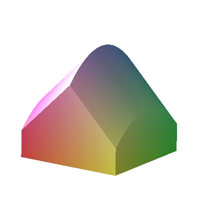
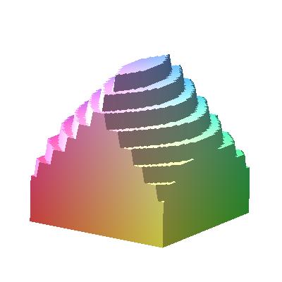
The next calculus course covers multivariable integration. Still, there are some higher dimensional things you can do with ordinary integrals. One of these is to compute a volume of an object if you know the area of its cross-sections. Dividing the object into \(n\) very thin slabs, the volume of the \(k^{th}\) one is roughly the thickness \(\Delta_k\) times the cross-sectional area of the \(k^{th}\) slab, call it \(A_k\text{;}\) see Figure 11.16.
The limit of \(\displaystyle\sum_{k=1}^n A_k \Delta_k\) should give the volume. Line up the slabs so that the \(x\)-axis goes perpendicular to the slabs. This limit looks awfully similar to the limit of \(\displaystyle\sum_{k=1}^n f(x_k) \Delta_k\) where \(x_k\) is any point on the \(x\)-axis inside the \(k^{th}\) slab and \(f\) is the function telling the cross-sectional area at every \(x\)-value. Therefore, the volume is computed by \(\displaystyle\int_a^b f(x) \, dx\) where \(a\) and \(b\) are the \(x\)-values at the first and last slab respectively.
Example 11.17. volume of a pyramid.
We write an integral for volume of a pyramid whose base is a square of side length \(s\) and whose height is \(h\text{.}\) It corresponds best to the description above if we orient it so the height is measured along the \(x\)-direction with the apex at the origin. See Figure 11.18. The cross-section is a square with side increasing linearly from 0 to \(s\) as \(x\) increases from 0 to \(h\text{.}\) Thus, the side length is given by \(\ell (x) = (s/h) x\text{,}\) hence the cross-sectional area is given by \(f(x) = (s/h)^2 x^2\) between \(x=0\) and \(x=h\text{.}\) The volume is therefore given by \(\displaystyle\int_0^h (s/h)^2 x^2 \, dx\text{.}\) When you learn to compute integrals, this will turn out to be a pretty easy one.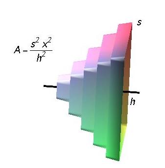
Subsection 11.4 The fundamental theorem of calculus
The reason we make such a fuss over integrals is that they can often be exactly computed. To see how this works, we look at the indefinite integral. Replacing the upper limit on the integral by a variable yields a function of that variable. To say this in another way, we may consider \(\displaystyle\int_a^b f(x) \, dx\) as a function of the free variables \(a\) and \(b\) (it can't be a function of \(x\) because \(x\) is a bound variable). Let \(a\) remain a constant but consider \(b\) to be a variable. We then have a function, \(b \mapsto \displaystyle\int_a^b f(x) \, dx\text{.}\) Denote this function by \(G\text{,}\) in other words \(G(b) := \displaystyle\int_a^b f(x) \, dx\text{.}\)
Example 11.19.
Let \(f (x) := 3x\) and \(a = 0\text{.}\) Then \(G(b) := \displaystyle\int_0^b 3x \, dx\text{.}\) Definite integrals compute area, hence \(G(b)\) is the area of the triangle with vertices at the origin, \((b,0)\) and \((b,3b)\text{.}\) The triangle area formula gives \(G(b) = (3/2) b^2\text{.}\)For fun (we have a warped sense of fun), compute \(G'\text{.}\) That's an easy one: \(G'(b) = 3b\text{.}\) Note that this is the integrand of the original integral, with the free variable \(b\) in place of the bound variable \(x\text{.}\) This is not a coincidence, as the following theorem asserts.
Theorem 11.20. Fundamental Theorem of Calculus.
Let \(f\) be a continuous function on an interval \([a,c]\text{.}\) For \(b \in (a,c)\text{,}\) let \(G(b) := \displaystyle\int_a^b f(x) \, dx\text{.}\) Then \(G'(b) = f(b)\text{.}\)Sketch of proof.
The derivative from the derivative from the right is given by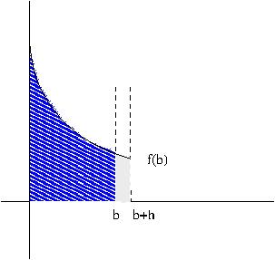
anti-derivatives.
The Fundamental Theorem of Calculus says we can evaluate integrals of \(f\) if we know a function \(G\) whose derivative is \(f\text{.}\) That motivates the next definition.
Definition 11.22.
An anti-derivative of a function \(f\) is any function \(G\) such that \(G' = f\text{.}\)How do we find anti-derivatives? The next chapter is entirely about computing these. Like rules for differentiation, rules for anti-differentiation start from a collection known results. For derivatives, we obtained these from the definition by computing limits. For anti-derivatives, we will get these simply by remembering some basic derivatives. The simple rule yielding the derivative of a polynomial may be run backwards. So for example the monomial \(a x^m\) has anti-derivative \(\frac{a}{m+1} x^{m+1}\text{.}\) We can sum these, obtaining the anti-derivative of any polynomial: an anti-derivative of \(\displaystyle\sum_{k=0}^m a_k x^k\) is given by \(\displaystyle\sum_{k=0}^m \frac{a_k}{k+1} x^{k+1}\text{.}\) In fact this works for negative or fracdtional powers, as long as the power is not \(-1\text{.}\)
Checkpoint 147.
We say "an anti-derivative" rather than "the anti-derivative" because for any given \(f\text{,}\) is always more than one anti-derivative. The functions \(G\) and \(G + c\text{,}\) where \(c\) is a constant, have the same derivative, so one is an anti-derivative of \(f\) if the other is. This is the only way anti-derivatives can differ. Once you know the value of the anti-derivative at any point, it is easy to reconstruct the correct anti-derivative as an integral, as in the following example.
Example 11.23.
Suppose \(G\) is an anti-derivative of \(f\) and \(G(3) = 7\text{.}\) We will look for an anti-derivative of the form \(G(b) = c + \displaystyle\int_a^b f(x) \, dx\text{.}\) To write \(G\) as an integral with a variable upper limit, begin by choosing the constant for the lower limit. The most convenient choice is 3, because we are supposed to know the value of \(G\) at 3. The function \(b \mapsto \displaystyle\int_3^b f(x) \, dx\) is zero at 3, so we will need to add 7. We therefore chooseCheckpoint 148.
What area is represented by the quantity \(G(7)\text{?}\)
Proposition 11.24. computing definite integrals with anti-derivatives.
The definite integral \(\displaystyle\int_a^b f(x) \, dx\) is equal to \(G(b) - G(a)\text{,}\) also denoted \(\left. G \right |_a^b\text{,}\) when \(G\) is any anti-derivative of \(f\text{.}\)Remark 11.25.
This implies that \(H(b) - H(a) = G(b) - G(a)\) when \(H\) is any other anti-derivative of \(f\text{.}\) In other words, differences of an anti-derivative at a specified pair of points do not depend on which particular anti-derivative was chosen.
Checkpoint 149.
Compute \(\displaystyle\int_1^6 x^2 - 5x + 6 \, dx\text{.}\)
\(\frac{6^{3}}{3}-\frac{5}{2}\cdot 6^{2}+36-\left(\frac{1}{3}-\frac{5}{2}+6\right)\)
Subsection 11.5 Estimating sums via integrals
We have seen integrals interpreted as areas and volumes, totals and averages, moments, and probabilities. One more use of an integral is to estimate a sum. In a way this is the reverse of the definition, which tells you that an integral is estimated by Riemann sums, in fact is a limit of such sums. Going the other way, if we have a sum, we can write an integral for which it is a Riemann sum. We may then expect the integral to be a good approximation for the sum. This will be easier when we know how to compute more integrals, but there are plenty we can already compute. We illustrate with a long example. It starts with the fact that the derivative of \(\ln x\) is \(1/x\text{.}\) This means that an anti-derivative of \(1/x\) is \(\ln x\text{.}\)Example 11.26. harmonic sum estimated by an integral.
Problem: estimate the \(100^{th}\) harmonic number \(1 + 1/2 + 1/3 + \cdots + 1/100\text{.}\) To solve this, we may as well estimate \(H_n := \displaystyle\sum_{k=1}^n 1/k\) for any positive integer \(n\text{.}\) Summing \(1/n\) looks a lot like integrating \(1/x\text{.}\) In fact, suppose we write a Riemann sum for \(\displaystyle\int_1^n 1/x \, dx\) that has precisely \(n-1\) rectangles. Then the intervals \(I_k\) are just the intervals \([1,2], [2,3], \ldots , [n-1,n]\text{.}\) Even better, we can make areas of the rectangles be exactly the same as in the sum. We just need to use the upper Riemann sum: \(1 + 1/2 + \cdots + 1/(n-1)\text{;}\) see the left-hand side of Figure 11.27 for a picture of this when \(n=9\text{.}\)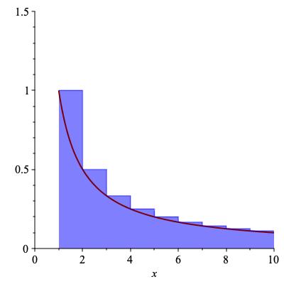
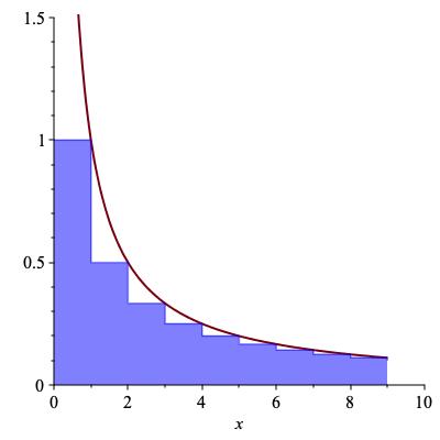
Figure 11.27 shows that \(H_{n-1}\) is an upper Riemann sum for \(\displaystyle\int_1^n 1/x \, dx\text{.}\) By Proposition 11.24 the integral is the difference of anti-derivatives:
Therefore, we have shown the bound \(H_{n-1} \geq \ln n\text{.}\) In particular, choosing \(n = 101\text{,}\) we see that \(H_{100} \geq \ln 101 \approx 4.615\text{.}\)
Is this an upper bound or a lower bound? It depends on your point of view. If we were trying to figure out the integral up to 100, \(H_{100}\) would be an upper bound on the value. But in this case we know the integral and are trying to estimate \(H_{100}\text{.}\) The integral provides a lower bound, in this case \(4.615\text{.}\)
What about an upper bound on \(H_{100}\text{.}\) The obvious thing is to see if we can make the same sum be a lower Riemann sum. Watch what happens when you try to do this. Take the graph, shift all the rectangles one unit left, and voilà! (See the right-hand side of Figure 11.27.) This shows that \(H_{100}\) is a lower Riemann sum for a slightly different integral, namely \(\displaystyle\int_0^{100} \frac{1}{x} \, dx\text{.}\) Alas, this is not an integral we can do because \(1 / x\) is not continuous at \(x=0\text{.}\) In fact, when we study improper integrals, we will see this evaluates to \(+ \infty\text{.}\) Sure, we get the upper bound \(H_{100} \leq \infty\text{,}\) but that is hardly useful. All is not lost, however, if we use some common sense. The same picture shows that an upper bound for the harmonic sum starting at 2 instead of 1 is
So, adding back the 1, we see that \(H_{100} \leq 1 + \ln 100 \approx 5.605.\) This is about as good as we can do with the techniques we have so far: \(4.615 \leq H_{100} \leq 5.605\text{.}\) For the record, \(H_{100} \approx 5.1874\text{.}\)
Trapezoidal approximation.
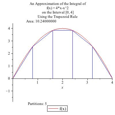
Sometimes it can be frustrating using Riemann sums because a lot of calculation doesn't get you all that good an approximation. You can see a lot of "white space" between the function \(f\) and the horzontal lines at the top of the rectangles that make up the upper or lower Riemann sum. If instead you let the rectangle become a right trapezoid, with both its top-left and top-right corner on the graph \(y = f(x)\text{,}\) then you get what is known as the trapezoidal approximation. The figure shows a trapezoidal approximation of an integral \(\displaystyle\int_0^4 f(x) \, dx\) with five trapezoids. Note that the first and last trapezoid are degenerate, that is, one of the vertical sides has length zero and the trapezoid is actually a right triangle. It is perfectly legitimate for one or more of the trapezoids to be degenerate.
Because the tops of the slices are allowed to slant, they remain much closer to the graph \(y = f(x)\) than do the Riemann sums. Because the area of a right trapezoid is the average of the areas of the two rectangles whose heights are the value of \(f\) at the two endpoints, it is easy to compute the trapezoidal approximation: it is just the average of the left-Riemann sum and the right-Riemann sum corresponding to the same partition into vertical strips.
Example 11.29.
Let's compute the trapezoidal approximation for \(\displaystyle\int_1^2 \frac{1}{1+x^2}\) with 10 trapezoids.
Averaging the left and right Riemann sums always gives a sum containing the \(n-1\) common terms plus half the first term for the left Riemann sum and the last term for the right Riemann sum. In this case one gets
The outcome of trapezoidal approximation in general can be summarized as,
Sum the values of \(f\) along a regular grid of \(x\)-values, counting endpoints as half, and multiply by the spacing between consecutive points.
The trapezoidal estimate is usually much closer than the upper or lower estimate, though it has the drawback of being neither an upper nor a lower bound. However, if you know the function to be concave upward then the trapezoidal estimate is an upper bound. Similarly if \(f'' \lt 0\) on the interval then the trapezoidal estimate is an lower bound. In the figure, \(f\) is concave downward and the trapezoidal estimate is indeed a lower bound.