Unit 4 Limits
You might not think limits would show up in a calculus course oriented toward application. Wrong! There are a lot of reasons why you need to understand the basic of limits. You should know these reasons, so here they are.
- You have already seen they show up in the definition of powers and logarithms when the exponent is not rational.
- The definition of derivative (instantaneous rate of change) is a limit.
- The number \(e \) is defined by a limit.
- Continuous compounding is a limit.
- Limits are needed to understand improper integrals, such as the integrals of probability densities.
- Infinite series, which we will discuss briefly, require limits.
- Discussing relative sizes of functions is really about limits.
Subsection 4.1 Definitions of limit
You should learn to understand limits in four ways:
- Intuitive
-
The limit as \(x \to a \) of \(f(x) \) is the numerical value (if any) that \(f(x) \) gets close to when \(x \) gets close to (but does not equal) \(a \text{.}\) This is denoted \(\lim_{x \to a} f(x) \text{.}\) If we only let \(x \) approach \(a \) from one side, say from the right, we get the one-sided limit \(\lim_{x \to a^+} f(x) \text{.}\)
Please observe the syntax: If I tell you a function \(f \) and a value \(a \) then the expression \(\lim_{x \to a} f(x) \) takes on a numerical value or "undefined". The variable \(x \) is a bound variable; it does not have a value in the expression and does not appear in the answer; it stands for a continuum of possible values approaching \(a \text{.}\) The variable \(a \) is free and does show up in the answer; for example \(\lim_{x \to a} x^2 \) is equal to \(a^2 \text{.}\)
- Pictorial
-
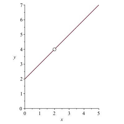
If the graph of \(f \) appears to zero in on a point \((a , b) \) as the \(x\)-coordinate gets closer to \(a \text{,}\) then \(b \) is the limit, even if the actual point \((a,b) \) is not on the graph. For example, suppose \(f(x) = \frac{x^2-4}{x-2} \text{.}\) Canceling the factor of \(x-2 \) from top and bottom, you can see this is equal to \(x+2 \text{,}\) except when \(x=2 \) because then you get zero divided by zero. Functions like this are not just made up for this problem. They occur naturally when solving simple differential equations, where indeed something different might happen if \(x=2 \text{.}\)
The graph of \(f \) has a hole in it, which we usually depict as an open circle, as in the left side of Figure 4.1. The value of \(\lim_{x \to 2} f(x) \) is 2, even though \(f\) is undefined precisely at 2.
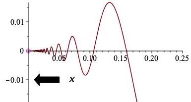
In this example the function \(f \) behaved very nicely everywhere except~2, growing steadily at a linear rate. The center figure shows the somewhat less well behaved function \(g(x) := x \sin(1/x) \text{.}\) This function is undefined at zero. As \(x \) approaches zero, the function wiggles back and forth an infinite number of times, but the wiggles are smaller and smaller. Intuitively, the value of the function \(g \) seems to approach zero as \(x \) approaches zero. Pictorially we see this too: zooming in on \(x=0 \) in the right-hand figure, corroborates that \(g(x) \) approaches zero.
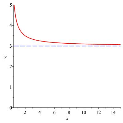
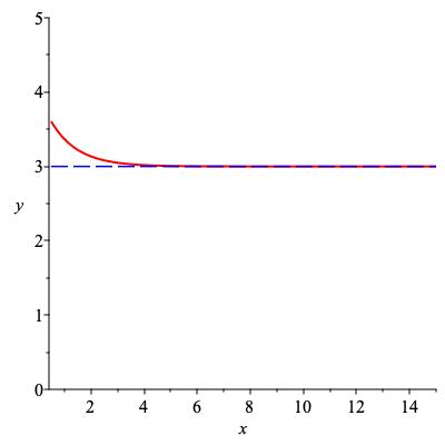
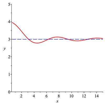
We can take limits at infinity as well as at a finite number. The limit as \(x \to \infty \) is particularly easy visually: if \(f(x) \) gets close to a number \(C \) as \(x \to \infty\) then \(f \) will have a horizontal asymptote at height \(C \text{.}\) Thus \(3 + \frac{1}{x} \text{,}\) \(3+e^{-x}\) and \(3 + \frac{\sin x}{x} \) all have limit 3 as \(x \to \infty \text{,}\) as shown in Figure 4.3.
- Formal
The precise definition of a limit is a little unexpected if you've never seen it before. We don't define the value of \(\lim_{x \to a} f(x) \text{.}\) Instead, we define when the statement \(\lim_{x \to a} f(x) = L \) is true. It can be true for at most one value \(L \text{.}\) If there is such a \(L \text{,}\) we call this the limit. If there is no \(L \text{,}\) we say the limit does not exist. When asked for the value of \(\lim_{x \to a} f(x) \text{,}\) you should answer with either a real number, or "DNE", for "does not exist". We won't have to spend a lot of time on the formal definition. You should see and grasp it at least once. Use of the Greek letters \(\varepsilon \) and \(\delta \) for the bound variables is a strong tradition.
- Computational
We'll focus a lot on how to compute limits, given a formula for a function or some other information about it. This involves rules which allow us to express a complicated limit in terms of several more straightforward limits.
Definition 4.4.
If \(f \) is a function whose domain includes an interval containing the real number \(a \text{,}\) we say that \(\lim_{x \to a} f(x) = L\) if and only if the following statement is true.
For any positive real number \(\varepsilon \) there is a corresponding positive real \(\delta \) such that for any \(x \) other than \(a \) in the interval \([a-\delta , a+\delta] \text{,}\) \(f(x) \) is guaranteed to be in the interval \([L - \varepsilon , L + \varepsilon] \text{.}\)
In symbols, the logical implication that must hold is:
Remark 4.5.
Loosely speaking, you can think of \(\varepsilon \) as an acceptable error tolerance in the \(y\) value and \(\delta \) as the precision with which you control the input (i.e., the \(x\) value). The limit statement says, you can meet even the pickiest error tolerance provided you can tune the input precisely enough.
Why is this a difficult definition? Chiefly because of the quantifiers. The logical form of the condition that must hold is: For all \(\varepsilon \gt 0 \) there exists \(\delta \gt 0 \) such that for all \(x \in [a-\delta , a+\delta] \text{,}\) \(\cdots \text{.}\) This has three alternating quantifiers (for all... there exists... such that for all...) as well as an if-then statement after all this. Experience shows that most people can easily grasp one quantifier "for all" or "there exists", but that two is tricky: "for all \(\varepsilon \) there exists a \(\delta \ldots\)". A three quantifier statement usually takes mathematical training to unravel.
Some people find it easier to conceive of the formal definition as a game. Alice is trying to show it's true. Bob is trying to show it's false. Alice says to Bob, no matter what \(\varepsilon \) you give me, I can find a \(\delta\) to make the implication true. (The implication is that all \(x\)-values fitting into Alice's \(\delta\)-interval will give values of \(f(x) \) inside Bob's interval.) Now they play the game: Bob tries to come up with a value of \(\varepsilon \) so small as to thwart Alice. Then Alice has to say her \(\delta \text{.}\) If she can always do so (assuming Bob has not made a blunder in overlooking the right choice of \(\varepsilon\)) she wins and the limit is \(L \text{.}\) If not (unless Alice has overlooked a \(\delta \) that would have worked), Bob has won and the limit is not \(L \text{.}\)
Subsection 4.2 Variations
Before introducing computational apparatus for limits, we need to finish the definitions by defining some variations: one-sided limits, limits at infinity and "limits of infinity" (which are in quotes because technically they are not limits at all).
One-sided limits.
Change the definition so that \(f(x) \) is only required to approach \(L\) when \(x \to a \) if \(x \) is greater than \(a \text{.}\) We say \(x \) "approaches \(a \) from the right," thinking of a number line. If the value of \(f(x) \) approaches \(L \) when \(x \) approaches \(a \) from the right, we say that the limit from the right of \(f(x) \) at \(x=a \) is \(L \text{,}\) and denote this \(\lim_{x \to a^+} f(x) = L \text{.}\) If we require \(f(x) \) to approach \(L \) when \(x \) approaches \(a \) but only for those \(x \) that are less than \(a \text{,}\) this is called having a limit from the left and is denoted \(\lim_{x \to a^-} f(x) = L \text{.}\)
Remark 4.6.
Just like wind directions (North wind, South wind, etc.), one-sided limits are named for the direction they come from, not the direction \(x \) is moving. Thus, \(\lim_{x \to 0^+} \) is evaluated by letting \(x \) approch zero from the positive direction, as shown to the right.
Checkpoint 40.
The lifetime of a light bulb is often modeled as a random variable with density \(f(x) = c e^{-c x}\) when \(x \geq 0\) and \(f(x) = 0\) when \(x \lt 0\) (light bulbs cannot have negative lifetimes). Here \(c\) is some positive constant. What are \(\lim_{x \to 0^+} f(x)\) and \(\lim_{x \to 0^-} f(x)\text{?}\)
\(\lim_{x \to 0^+} f(x)=\)
\(\lim_{x \to 0^-} f(x)=\)
Checkpoint 41.
Both kinds of one-sided limits require something less stringent, so the statement \(\lim_{x \to a} f(x) = L \) automatically implies both \(\lim_{x \to a^+} f(x) = L \) and \(\lim_{x \to a^-} f(x) = L \text{.}\) Likewise, if \(f(x) \) is forced to approach \(L \) when \(x \) approaches \(a\) from the right, but also when \(x \) approaches \(a \) from the left, then this covers all \(x \text{,}\) and the (unrestricted) limit will be \(L \text{.}\) If you want, you can summarize this as a theorem -- wait, no it's too puny, let's make it a proposition. We won't be referring to this too often, but here it is.
Proposition 4.7.
For every function \(f \) and real numbers \(a \) and \(L \text{,}\)Checkpoint 42.
Suppose \(f\) is a function satisfying \(\lim_{x \to 4^-} f(x) = 2\) and \(\lim_{x \to 4^+} f(x) = 1 \text{.}\)
Sketch a graph of such a function.
What is \(\lim_{x \to 4} f(x)\text{?}\)
\(\text{DNE}\)
Example 4.8.
Let \(f(x) = \lfloor x \rfloor \text{,}\) the greatest integer function. Let's evaluate the one-sided limits and two-sided limit at a couple of values. First, take \(a = \pi \text{,}\) you know, the irrational number beginning \(3.14\ldots \text{.}\) If we just look near this value, say between \(3.1 \) and \(3.2 \text{,}\) it is completely flat: a constant function, taking the value~3 everywhere. So of course the limit at \(x=\pi \) will also be~3. This is the same by words or pictures; see Figure 4.9.
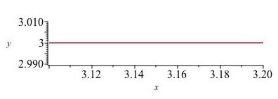
By the formal definition, no matter what \(\varepsilon \) is chosen, you can take \(\delta = 0.1 \text{,}\) say, and \(f(x) \) will be within \(\varepsilon \) of~3 because it will be exactly~3. So the limit is~3, hence so are both one-sided limits as in the picture just above.
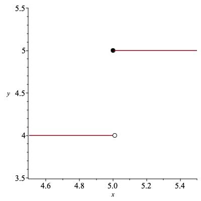
Now take \(x \) to be an integer, say \(a=5 \text{.}\) The limit from the right looks like it did before, with \(f(x) \) taking the value~5 for every sufficiently close \(x \) (here sufficient means within~1) greater than~5. On the other hand, when \(x \) is close to~5 but less than~5, we will have \(f(x) = 4 \text{,}\) as in the picture below. Thus,
The two-sided limit does not exist because the two one-sided limits are not equal; see Figure 4.10.
Checkpoint 43.
Let \(f(x) = \text{sgn} (x) \text{,}\) the sign function. Use the verbal, pictorial or formal definition, as you please, to give values of these limits. If the limit does not exist, enter “DNE”. You can use “inf” to stand for \(\infty\) if needed.
\(\lim_{x \to 0^+} f(x)\)
\(\lim_{x \to 0^-} f(x)\)
\(\lim_{x \to 0} f(x)\)
How about if we take the absolute value: is \(\lim_{x \to 0} |\text{sgn}(x)|\) any different?
yes; the limit for |sgn| is 0
yes; the limit for |sgn| is 1
yes; the limit for |sgn| does not exist
no, the limit for |sgn| does not exist
Limits at infinity.
You have already seen the pictorial and verbal version of a limit at infinity. Here is the formal definition. It repeats a lot of the definition of a limit at \(x=a \text{.}\) The only difference is that instead of having to come up with an interval \([a-\delta , a+\delta]\) guaranteeing \(f(x) \) is within \(\varepsilon \) of the limit, you have to come up with an "interval near infinity". This turns out to mean an interval \([M,\infty) \text{.}\) In other words, there must be a real number \(M \) guaranteeing \(f(x) \) is with \(\varepsilon \) of \(L \) when \(x \gt M \text{.}\)
Remark 4.11.
Informally, "close to infinity" turns into "sufficiently large". In the tolerance/accuracy analogy, getting \(f(x) \) to be close to \(L\) to within the acceptable tolerance will result from guaranteed largeness of the input rather than guaranteed closeness to \(a \text{.}\)
Definition 4.12.
We say that \(\lim_{x \to \infty} f(x) = L \) if and only if \(L \) is a real number and:For any positive real number \(\varepsilon \) (think of this as acceptable tolerance in the \(y \) value) there is a corresponding real \(M\) (think of this as guaranteed minimum value for \(x\)) such that for any \(x \) greater than \(M \text{,}\) \(f(x) \) is guaranteed to be in the interval \([L - \varepsilon , L + \varepsilon] \text{.}\)
In symbols, the logical implication that must hold is:
If a real number \(L \) exists satisfying this, we write \(\lim_{x \to \infty} f(x) = L \text{.}\) Sometimes to be completely unambiguous, we put in a plus sign: \(\lim_{x \to +\infty} f(x) = L \text{.}\)
Checkpoint 44.
True or false?
true
false
\(\text{false}\)
Limits at \(-\infty \) are defined exactly the same except for a single inequality that is reversed. Now the implication that must hold is that for some (possibly very negative) \(M \text{,}\)
When this holds, we write \(\lim_{x \to -\infty} f(x) = L \text{.}\) When no such \(L \) exists, we write \(\lim_{x \to -\infty} f(x) \) DNE.
Example 4.13.
Let \(f(x) := \frac{x}{\sqrt{1+x^2}} \text{.}\) Because \(\sqrt{1+x^2} \) is a little bigger than \(|x| \) but almost the same when \(x \) or \(-x \) is large, this function satisfies
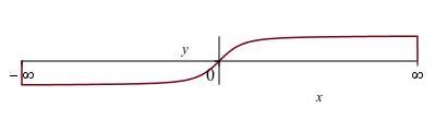
The graph of this function is shown in Figure 4.14. It has horizontal asymptotes at 1 and \(-1 \text{.}\) This suggests how to define a horizontal asymptote.
Definition 4.15.
A function \(f \) or its graph is said to have a horizontal asymptote at height \(b \) if \(\lim_{x \to \infty} f(x) = b \) or \(\lim_{x \to - \infty} f(x) = b \text{.}\)
Checkpoint 45.
- Sketch a graph of a function \(f \) for which \(\lim_{x \to -\infty} f(x) \) exists but \(\lim_{x \to +\infty} f(x) \) does not.
- Give a formula defining a function \(g(x) := \cdots \) such that \(\lim_{x \to -\infty} g(x) \) exists but \(\lim_{x \to +\infty} g(x) \) does not.
- Which of these two things was easier to do?
"Limits" of infinity.
Consider the function \(f(x) = 1/x^2 \text{,}\) defined for all real numbers except zero. What happens to \(f(x) \) as \(x \to 0\text{?}\) By our definitions, \(\lim_{x \to 0} 1/x^2 \) does not exist. But we can see that \(f(x) \) "goes to infinity". Because infinity is not a number, the limit technically does not exist. However, it is useful to classify DNE limits as ones where the function approaches \(\infty \) (or \(-\infty\)) versus ones where there is no consistent behavior.
Remark 4.16.
This time, instead of staying within a tolerance of \(\varepsilon \) in the output, we make the output sufficiently large (greater than any given \(N\)) or small. We do this by guaranteeing \(\delta \) accuracy in the input (for limits as \(x \to a\)) or by making the input sufficiently large or small (limits as \(x \to \pm \infty\)).
Formally, this turns into the following defintion.
Definition 4.17.
If \(f \) is a function and \(a \) is a real number, we say that \(\lim_{x \to a} f(x) = +\infty \) if for every real \(N \) there is a \(\delta \gt 0 \) such that \(0 \lt \left\lvert x-a\right\rvert \lt \delta \) implies \(f(x) \gt N \text{.}\)
Again, if we reverse the last inquality to require that \(f(x) \lt N\) (and \(N \) can be a very negative number) we get the definition for a limit of negative infinity. Please remember these are all subcases of limits that don't exist! If you show that a limit is infinity, you have shown that the limit does not exist (and you have specified a particular reason it doesn't exist).
Example 4.18.
Let's check that \(\lim_{x \to 0} 1/x^2 = +\infty \text{.}\) Given a positive real number \(N \text{,}\) how can we ensure \(f(x) \gt N\text{?}\) Answer: for positive numbers, \(f \) is decreasing and \(f(x) = N\) precisely when \(x = 1 / \sqrt{N} \text{.}\) Therefore, if we keep \(x \) positive but less than \(1 / \sqrt{N} \) then \(f(x) \) will be greater than \(N \text{.}\) We have just shown that \(\lim_{x \to 0^+} 1/x^2 = +\infty \text{.}\) Similarly, when \(x \) is negative, if we keep \(x \) in the interval \((-1/\sqrt{N}, 0) \) we ensure \(1/x^2 \gt N \text{.}\) So \(\lim_{x \to 0^-} \) is also \(+\infty \text{.}\) Both one-sided limits are \(+\infty \text{,}\) therefore
Don't forget, it follows from the limit being \(+\infty \) that
For one-sided limits and limits at infinity, the DNE case also includes a case where the limit would be said to be infinity. Stating all these would be repetitive. Try one, to make sure you agree it's straightforward.
Checkpoint 46.
Write a formal definition for the statement \(\lim_{x \to a^+} f(x) = -\infty \text{.}\)
Checkpoint 47.
Consider the function \(1/x \text{.}\) What should we say about \(\lim_{x \to 0^+} 1/x \) and \(\lim_{x \to 0^-} 1/x \text{?}\) If the limit does not exist, enter "DNE". You can use "inf" to stand for \(\infty\) if needed.
\(\lim_{x \to 0^+} 1/x\)
\(\lim_{x \to 0^-} 1/x\)
Limit of a sequence.
A special case of limits at infinity is when the domain of \(f\) is the natural numbers. When \(f \) is only defined at the arguments \(1, 2, 3, \ldots \text{,}\) it is more usual to think of it as a sequence \(b_1, b_2, b_3, \ldots \text{,}\) where \(b_k := f(k) \text{.}\) The definition of a limit at infinity can be applied directly, resulting in the definition of the limit of a sequence.
Definition 4.19.
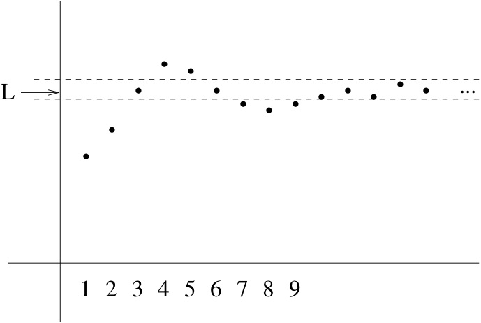
[limit of a sequence]Given a sequence \(\{ b_n \} \) and a real number \(L \) we say \(\lim_{n \to \infty} b_n = L \) if and only if for all \(\varepsilon \gt 0\) there is an \(M \) such that \(|b_n - L| \lt \varepsilon \) for every \(n \gt M \text{.}\)
Remark 4.20.
Often we use letters such as \(n \) or \(k \) to denote integers and \(x \) or \(t \) to denote real numbers. Therefore, by context, \(\lim_{n \to \infty} 1/n \) denotes the limit of a sequence while \(\lim_{t \to \infty} 1/t \) denotes the limit at infinity of a function. Formally we should clarify and not count on the name of a variable to signify anything! But because the two definitions agree, often we don't bother.
Checkpoint 48.
Pictorially, if a sequence has a limit \(L \text{,}\) then for every pair of parallel horizontal lines, however narrow, enclosing the height \(L \text{,}\) the sequence must eventually stay between them. This is shown in Figure 4.21.
As you will see, Proposition 4.27 and Proposition 4.28 give ways to determine limits of more complicated functions once you understand limits of some basic functions. Here is another piece of logic that can help do the same thing. You will prove it in your homework.
Theorem 4.22.
Let \(a \) be a real number or \(\pm \infty \) and let \(f, g \) and \(h \) be functions satisfying \(f(x) \leq g(x) \leq h(x) \) for every \(x \text{.}\) If \(\lim_{x \to a} f(x) = L \) and \(\lim_{x \to a} h(x) = L \) then also \(\lim_{x \to a} g(x) = L \text{.}\) If we know only that \(\lim_{x \to a^+} h(x) = \lim_{x \to a_-} h(x) = L \) then we can conclude \(\lim_{x \to a^+} g(X) = L \text{,}\) and same for limits from the left.The same fact is true of sequences: if \(a_n \leq b_n \leq c_n\) for these three sequences and the first and last sequence converge to the same limit \(L \text{,}\) then so does the middle one. We will not do anything with this now, but will get back to this fact in a week or two. The next exercise brushes up on the logical syntax of limits.
Checkpoint 49.
Evaluate the limits:
\(\lim_{x \to {5}} c x=\) .
\(\lim_{t \to a} b t =\) .
In each of these two cases, say which variables (any letter appearing in the expression other than letters spelling “lim”) are free and which are bound.
\(x\text{:}\)
free
bound
free
bound
\(t\text{:}\)
free
bound
free
bound
free
bound
In comparing your answers to the first part and the second part, what do you notice?
Subsection 4.3 Continuity
Definition 4.23.
A function \(f \) is said to be continuous at the value \(a \) if the limit exists and is equal to the function value, in other words, if \(\lim_{x \to a} f(x) = f(a) \text{.}\)
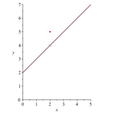
Intuitively, this means the limit at \(a \) exists and there is no hole: the function is actually defined at \(a \) and wasn't given some weird other value. To illustrate what we mean, consider this picture of a function that is discontinuous at \(x=2 \) even though \(\lim_{x \to 2} f(x) \) exists and so does \(f(2) \text{,}\) because the values don't agree.
Checkpoint 50.
Is \(\lim_{x \to a} f(x) - f(a) = 0\) the same as \(f\) being continuous at \(a\text{?}\)
yes, these mean the same thing
no, these are different ideas
Explain.
\(\text{yes, ... same thing}\)
Continuity on regions.
Definition 4.25.
A function is said to be continuous on an open interval \((a,b) \) if it is defined and continuous at every point of \((a,b) \text{.}\)
A function is said to be continuous on an closed interval \((a,b) \) if it is defined and continuous at every point of \((a,b) \text{,}\) with only one-sided contintuity required at \(a^+ \) and \(b_- \text{.}\)
A function \(f \) is said to be just plain continuous if it is continuous on the whole real line.
Checkpoint 51.
Which of the basic trig functions \(\sin \text{,}\) \(\cos\) and \(\tan\) are continuous on \((0, 2\pi)\text{?}\) You don’t need to prove your answer, just to have an intuitive justification in mind.
\(\displaystyle \sin\)
\(\displaystyle \tan\)
\(\displaystyle \cot\)
\(\displaystyle \sec\)
\(\displaystyle \csc\)
\(\text{Choice 1}\)
Before going on to use the notion of continuity to help us compute limits, we will state one famous result which will seem either stupid and obvious or deep and tricky.
Theorem 4.26. Intermediate Value Theorem.
Let \(f \) be a continuous function defined on the closed interval \([a,b]\) and suppose that \(y \) is any value between the values \(f(a) \) and \(f(b) \text{.}\) Then there is some number \(c \) in the interval \([a,b] \) satisfying \(f(c) = y \text{.}\)This says, basically, a continuous function can't get from one value to another without hitting everything in between. The theorem is most often used when there is a number we can only define this way. For example, let \(f(x) := e^x / x \text{,}\) which is an increasing function on the half-line \([1,\infty) \text{.}\) We want to say "let \(c \) be the value for which \(f(c) = 3 \text{.}\)" How do we know there is one? Well, \(f(1) = e \text{,}\) which is less than 3, and \(f(3) \approx 6.695 \) which is greater than 3. So there must be an argument between 1 and 3 where \(f \) takes value 3. There can be only one because \(f \) is strictly increasing (you can prove after another two sections).
Subsection 4.4 Computing limits
Computing a limit by verifying the formal definition is a real pain. There is computational apparatus that allows us to compute limits of many functions once we know limits of a few simple ones. One approach we have seen in textbooks is to give a list of rules that work. It looks something like this.
Proposition 4.27.
If \(\lim_{x \to a} f(x) = L \) and \(c \) is a real number thenProposition 4.28.
If \(f \) and \(g \) are functions and \(a,K,L \) are real numbers with \(\lim_{x \to a} f(x) = K \) and \(\lim_{x \to a} g(x) = L \text{,}\) thenExample 4.29.
Suppose \(f \) is a polynomial: \(f(x) = b_n x^n + \cdots + b_1 x + b_0 \text{.}\) What is \(\lim_{x \to a} f(x)\text{?}\) We hope you think this is a really boring example. Of course, the polynomial is continuous (picture in your mind the graph of a polynomial) and so we expect \(\lim_{x \to a} f(x) = f(a) \text{.}\) But why?
First note that we can evaluate the limit at \(a\) of the monomial \(x^k \) as \(a^k \) using the second conclusion of Proposition 4.27. We can evaluate the limit at \(a\) of each monomial \(b_k x^k \) as \(b_k a^k \) by applying the first conclusion of Proposition 4.27 with \(c = b_k \) and \(f(x) = x^k \text{.}\)
So each term in the polynomial has the right behavior. We still need to combine them all by addition. This is allowed to us by Proposition 4.28.
The fact that polynomial limits can be computed just by "plugging in" the value \(x=a\) comes up a lot, so we record it as a propostion.
Proposition 4.30.
Polynomials are continuous. The limit of a polynomial \(f \) at \(a\) is always given by \(f(a) \text{.}\)Checkpoint 52.
Checkpoint 53.
So that Proposition 4.27 Proposition 4.28 don't look like arbitrary rules from out of nowhere, you should realize they can be proved, and in fact follow from one basic theorem.
Theorem 4.31.
If the function \(f \) has a limit \(L \) at \(x=a \) and the function \(H \) is continuous at \(L \) then \(H \circ f \) will have the limit \(H(L) \) at \(x=a \text{.}\) Formally,Why do the Proposition 4.27 and Proposition 4.28 follow from this principle? Let \(H(x) \) be the continuous function \(c x \text{.}\) Then \(H \circ f \) is \(c f(x) \) and we recover the first conclusion of Proposition 4.27. Setting \(H(x) := x^c \) recovers the second conclusion.
Checkpoint 54.
A related fact about limits is computation by change of variables. Suppose \(g\) is a function such that \(\lim_{x \to 0} g(x) = {-1} \text{.}\) What is \(\lim_{x \to 0} g(2x)\text{?}\)
Explain in words.
\(-1\)
Checkpoint 55.
Some more techniques and tricks.
This course is more about using limits than it is about computational technique, but you should at least see some of the standard techniques for cases that go beyond what's in Proposition 4.27 and Proposition 4.28.
Suppose you need to evaluate \(\lim_{x \to a} f(x) / g(x) \text{.}\) If both \(f \) and \(g \) have nonzero limits at \(a \text{,}\) say \(L \) and \(M \text{,}\) then Proposition 4.28 tells you
In fact if \(L=0 \) but \(M \neq 0 \text{,}\) this still works. If \(M=0 \) but \(L\neq 0 \text{,}\) then the question of evaluating \(\lim_{x \to a} f(x) / g(x) \) also has an easy answer.
Checkpoint 56.
The remaining case, when \(L = M = 0 \text{,}\) can be enigmatic. Calculus provides one solution you will see in a few weeks (L'Hôpital's Rule), but you can often solve this with algebra. If you can factor out \((x-a) \) from both \(f \) and \(g \text{,}\) you may get a simpler expression for which at least one of the functions has a nonzero limit.
Example 4.32.
What is
Both numerator and denominator are continuous functions with values of zero (hence limits of zero) at~5. That suggests dividing top and bottom by \(x-5 \text{,}\) resulting in \(\lim_{x \to 5} \frac{x + 5}{x} \text{.}\) Both numerator and denominator are continuous functions so we can just evaluate and get \(10 / 5 \) so the answer is 2.
Sometimes you have to do a little algebra to simplify. Here's an example of one of the most common simplification tricks.
Example 4.33.
What is \(\lim_{x \to 0} \frac{\sqrt{x+1} - 1}{x}\text{?}\) Multiplying and dividing by the so-called conjugate expression, where a sum is turned into a difference or vice versa, gives
The numerator and denominator are continuous at \(x=0 \) with nonzero limits of 1 and 2 respectively, so the limit is equal to \(1/2 \text{.}\)
This algebra trick occurs so commonly throughout mathematics that you should always think about conjugate radicals every time you see an expression with a square root added to or subtracted from something!
Further tricks can wait until you've learned some more background. Although limits are needed to define derivatives, you can then use derivatives to evaluate more limits (L'Hôpital's Rule). Similarly, limits are used to define orders of growth, which can then be used to evaluate more limits.