CHAPTER 6 - Transcendental Functions

Section 6.1, page 454

Problem 31

We are given the function, and asked to find the derivative of its inverse at the point where

x=-1. We'll call the inverse function finv(x) We are also told (though we will solve for it here) that -1 = f(3). We'll start by writing the equation that defines the inverse function:

>	eqn:=x=finv(x)^3-3*finv(x)^2-1;

>	rts:=solve(subs(x=-1,eqn),finv(-1));

Since we're only interested in values bigger than 2, we see that we should take finv(-1)=3. We could use the rule to calculate the derivative, but we'll just take the derivative of both sides of the equation:

>	deqn:=diff(eqn,x);

Now we'll solve this for the derivative of finv:

>	solve(deqn,diff(finv(x),x));

Finally, we'll substitute what we know: that finv(-1)=3. This will give us d finv/dx at x=-1.

>	subs(finv(x)=3,%);

Let's compare this with the "formula way" -- we should just take 1/y' evaluated at -1:

>	1/subs(x=3,diff(x^3-3*x^2-1,x));

(see the Math 103 solved problems for more from this section)

Section 6.2, page 465

Problem 82

To solve this second-order differential equation, we'll integrate twice (be sure to add the +C each time!):

>	dy:=int(sec(x)^2,x)+C;

>	y:=int(dy,x)+K;

Now we'll apply the initial conditions: y(0)=0 and y'(0)=1:

>	simplify(solve({subs(x=0,y)=0,subs(x=0,dy)=1},{C,K}));

Well, we know that cos(0)=1 even if Maple doesn't seem to. So we put K=0, C=1 into y for the final answer:

>	y:=subs(K=0,C=1,y);

(see the Math 103 solved problems for more from this section)

Section 6.3, page 472

Problem 20

An easy one!

>	diff(exp(4*sqrt(x)+x^2),x);

Problem 40

This is an implicit differentiation problem:

>

restart;

>	eqn:=tan(y(x))=exp(x)+ln(x);

>	solve(diff(eqn,x),diff(y(x),x));

Problem 63

Another initial value problem. We'll solve this one using dsolve:

>	dsolve({diff(y(t),t)=exp(t)*sin(exp(t)-2),y(ln(2))=0},y(t));

(see the Math 103 solved problems for more from this section)

Section 6.4, page 480

Problem 8

>	solve(8^(log[8](3))-exp(ln(5))=x^2-7^(log[7](3*x)),x);

Problem 27

>	simplify(diff(log[2](r)*log[4](r),r));

Problem 51

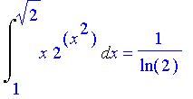
>	Int(x*2^(x^2),x=1..sqrt(2))=int(x*2^(x^2),x=1..sqrt(2));

Problem 85

"Tangent line" idiom!

>	f:=2^x; tanline:=subs(x=0,f)+subs(x=0,diff(f,x))*(x-0);

>	evalf(tanline);

part (b)

>	plot({f,tanline},x=-3..3,color=blue,thickness=2);

>	plot({f,tanline},x=-1..1,color=blue,thickness=2);

Section 6.5, page 488

Problem 8

Exponential growth implies that:

>	pop:=P*exp(k*t);

The data we're given allow us to solve for k and P

>	solve({subs(t=3,pop)=10000,subs(t=5,pop)=40000},{P,k});

Obviously only the first one of these makes sense. And P=1250 is the answer to our problem, since it asks for the number of bacteria present initially.

Problem 12

(a) The price p per unit ordered depends on the number x of units ordered according to the differential equation

>	deqn:=diff(p(x),x)=-0.01*p(x);

And we know that p(100)=20.09. So we have the initial condition

>	init:=p(100)=20.09;

We can apply dsolve to this:

>	dsolve({deqn,init},p(x));

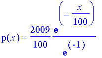
>	p:=simplify(rhs(%));

(b) Some sample prices: For 10 unit and 90 unit orders:

>	evalf(subs(x=10,p)),evalf(subs(x=90,p));

(c),(d)  Revenue = x*p -- we'll graph first, then find the max:

>	rev:=x*p; plot(rev,x=0..120,color=blue,thickness=2);

>	solve(diff(rev,x)=0,x);

Section 6.6, page 496

Problem 35

(Maple knows limits):

>	Limit(1/(x-1)-1/ln(x),x=1,right)=limit(1/(x-1)-1/ln(x),x=1,right);

Problem 65

(a) First the verification:

>	Limit((1+1/x)^x,x=infinity)=limit((1+1/x)^x,x=infinity);

(b) We'll make a sequence of larger and larger x's and values of :

>	f:=(1+1/x)^x;

>	seq([10^k,evalf(subs(x=10.0^k,f))],k=1..15);

Something happened around 10^9 -- we fell victim to round-off error. To go farther, we can have Maple keep more decimal places as follows:

>	Digits:=20;

>	seq([10^k,evalf(subs(x=10.0^k,f))],k=1..15);

>	evalf(exp(1));

So we're getting pretty close. Let's try graphing, as suggested in the text:

>	Digits:=10;

>	plot(f,x=1..10^10);

That looks good -- perhaps we can go farther:

>	plot(f,x=10^10..10^12);

So we see the roundoff problem begin to emerge.

Section 6.7, page 503

Problem 8

We'll check this by taking limits of quotients:

>	limit(2^x/x^2,x=infinity);

>	limit(ln(2)^x/2^x,x=infinity);

>	limit(ln(2)^x/x^2,x=infinity);

>	limit(exp(x)/2^x,x=infinity);

So we have  <  when x goes to infinity (in fact,

>	limit(ln(2)^x,x=infinity);

so it doesn't grow at all!)

Section 6.8, page 510

Problem 19

>	simplify(tan(arcsin(-1/2)));

Problem 29

>	simplify(sec(arctan(x/2)));

Problem 44

>	Limit(arctan(x),x=-infinity)=limit(arctan(x),x=-infinity);

Section 6.9, page 518

Problem 36

>	Int(6/sqrt(4-(r+1)^2),r)=int(6/sqrt(4-(r-1)^2),r);

Problem 58

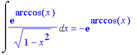
>	Int(exp(arccos(x))/sqrt(1-x^2),x)=int(exp(arccos(x))/sqrt(1-x^2),x);

Section 6.11, page 537

Problem 10

We'll apply "dsolve"

>	eqn:=(y(x)+1)*diff(y(x),x)=y(x)*(x-1);

>	dsolve(eqn,y(x));

Maple has solved explicitly even though you might not have been able to. In fact, after separating, you'd get:

>	int((y+1)/y,y)=int(x-1,x)+C;

>	solve(%,y);

which differs from the dsolve solution by the definition of the constant.

Problem 16

>	eqn:=exp(x)*diff(y(x),x)+2*exp(x)*y(x)=1;

>	dsolve(eqn,y(x));

Problem 40

An initial-value problem:

>	eqn:=diff(y(x),x)+x*y(x)=x; init:=y(0)=-6;

>	dsolve({eqn,init},y(x));

Problem 46

First set up and solve the initial-value problem:

>	eqn:=diff(x(t),t)=1000+0.1*x(t); init:=x(0)=1000;

>	dsolve({eqn,init},x(t));

The question in part (b) is when will this equal 100000:

>	solve(rhs(%)=100000,t);

>

evalf(%);

So it takes about 23 years to get to $100,000.

Section 6.12, page 545

Problem 3

Maple has numerical DE solvers, but they are more sophisticated than Euler's method. If we really want to use Euler's method, we have to write it ourselves as follows: If the equation is y ' = f(x,y), then we'll define f first, then set

>	eul:=(x,y,h)->y+h*f(x,y);

This will give the next value of y. So for this problem we'd get:

>	f:=(x,y)->2*x*y+2*y;

>	eul(0,3,0.2);

So y(0)=3, and y(0.2)=4.2. Next,

>	eul(0.2,4.2,0.2);

>	eul(0.4,%,0.2);

And so forth. Our first four points are [0,3], [0.2,4.2], [0,4,6.216], [0.6,9.69696].

Problem 18

We use the DEplot command in the DEtools library (see the section in the manual on this command for more details):

>	with(DEtools,DEplot):

>	DEplot(diff(y(x),x)=2*(y(x)-4),y(x),x=-2..2,y=-3..8,{[0,1],[0,4],[0,5]},thickness=2,color=blue,linecolor=black);