Worked Sample Problems - Math 104
CHAPTER 5 - Applications of Integrals
Section 5.1, page 371
Problem 26
Since the curves have x as functions of y, rather than the other way around, we'll use "implicitplot" to plot them:
| > | with(plots,implicitplot): |
| > | eqn1:=x-y^2=0; eqn2:=x+2*y^2=3; |
![]()
![]()
Before we plot, we solve for where the curves intersect (so we plot in the right place):
| > | solve({eqn1,eqn2},{x,y}); |
![]()
OK:
| > | implicitplot({eqn1,eqn2},x=-2..4,y=-2..2,color=blue,thickness=2); |
![[Maple Plot]](images/m104-ex54.gif)
To calculate the area, we'll take a rectangle of height dy and width from the left curve to the right:
| > | x1:=solve(eqn1,x); x2:=solve(eqn2,x); |
![]()
![]()
The rectangles will touch x1 on the left and x2 on the right. So the area is:
| > | area:=int(x2-x1,y=-1..1); |
![]()
(see the Math 103 solved problems for more from this section)
Section 5.2, page 377
Problem 10
We'll start by drawing the solid -- this is a nice exercise in visualization and 3-D geometry. Be sure to come back and look at it when you're studying multivariable calculus.
The base of the solid is the circle 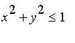 -- and the cross sections are 45-45-90 triangles with one leg parallel to the x-axis in the base. For a given value of y, this leg has length
  , and so the three vertices of the right triangle are [
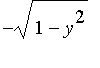 ,y,0], [
 ,y,0], and [
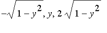 ]. Calculating the volume of this solid will be easy, compared to drawing it.
The boundary of the solid has three pieces: the bottom, a vertical side (where the second legs of the triangles are) and a slanted side (the hypotenuses of the triangles). Here's how to draw it:
| > | plot3d({[-sqrt(1-u^2),u,v*2*sqrt(1-u^2)],[sqrt(1-u^2)-2*v*sqrt(1-u^2),u,v*2*sqrt(1-u^2)],[sqrt(1-u^2)-2*v*sqrt(1-u^2),u,0]},u=-1..1,v=0..1,scaling=constrained); |
![[Maple Plot]](images/m104-ex513.gif)
In the Maple version of this worksheet on the web, you can grab the solid and turn it in different directions to get a better feel for it.
Now for the volume computation: We slice perpendicular to the y-axis. So the slices have width dy, and they are 45-45-90 triangles with base and height both equal to 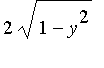 . So the volume of the solid is
| > | volume:=int(1/2*2*sqrt(1-y^2)*2*sqrt(1-y^2),y=-1..1); |
Section 5.3, page 385
Problem 38
(a) The region we're talking about is
| > | plot({[x,2*x,x=0..1],[x,0,x=0..1],[1,y,y=0..2]},color=blue,thickness=2,view=[0..3,0..3]); |
![[Maple Plot]](images/m104-ex516.gif)
The solid obtained by rotating this around the line x=1 is:
| > | with(plots,tubeplot): |
| > | tubeplot([1,y,0],y=0..2,radius=1-y/2,tubepoints=18,color=black,style=hidden,orientation=[-90,5],axes=normal); |
![[Maple Plot]](images/m104-ex517.gif)
To get its volume, we'll use disks -- for each y between 0 and 2, the disk has radius 1-y/2. So the volume is
| > | vol1:=int(Pi*(1-y/2)^2,y=0..2); |
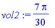
(b) Now we revolve around the line x=2. This solid looks like this:
| > | with(plots,display3d): |
| > | A:=tubeplot([2,y,0],y=0..2,radius=2-y/2,tubepoints=18,color=black,style=hidden,orientation=[-90,25],axes=normal): |
| > | B:=tubeplot([2,y,0],y=0..2,radius=1,tubepoints=18,color=black,style=hidden): |
| > | display3d({A,B}); |
![[Maple Plot]](images/m104-ex519.gif)
So you can see that there is a hole in the middle. So we'll use washers this time, with inner radius 1 and outer radius 2-y/2. So the volume is
| > | vol2:=int(Pi*(2-y/2)^2-Pi*1^2,y=0..2); |
(see the Math 103 solved problems for more from this section)
Section 5.4, page 392
Problem 26
First, we'll graph the region:
| > | implicitplot(x=y-y^3,x=0..2,y=0..2,color=blue,thickness=2); |
![[Maple Plot]](images/m104-ex521.gif)
(a) If we revolve this around the x-axis, it's easier to calculate the volume using cylindrical shells, of radius y, thickness dy and "height" (width)  . We do this as follows:
| > | vol1:=int(2*Pi*y*(y-y^3),y=0..1); |
(b) If we revolve this around the y-axis, it's again easier to use shells, but now for each y between 0 and 1 the radius is 1-y, the thickness is still dy and the height is still  . So we get:
| > | vol2:=int(2*Pi*(1-y)*(y-y^3),y=0..1); |
They're not the same (so that curve isn't quite as symmetric about the line y=1/2 as it looks!)
Section 5.5, page 398
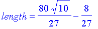
Problem 10
We'll just do it:
| > | y:=x^(3/2); |

| > | length=int(sqrt(1+diff(y,x)^2),x=0..4); |
Section 5.6, page 405
Problem 15
Since we're going around the x axis, the surface area element is 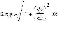 . So we integrate:
| > | y:=sqrt(2*x-x^2); |
![]()
| > | surfarea:=int(2*Pi*y*sqrt(1+diff(y,x)^2),x=1/2..3/2); |
![]()
Section 5.7, page 416
Problem 26
Let's draw the plate first:
| > | y1:=x^2; y2:=x; |
![]()
![]()
| > | plot({y1,y2},x=-0.2..1.2,color=blue,thickness=2); |
![[Maple Plot]](images/m104-ex533.gif)
We find the mass and the moments around the x and y axes:
| > | density:=12*x; |
![]()
| > | mass:=int(density*(y2-y1),x=0..1); |
![]()
To get the moment around the y axis, use vertical strips:
| > | My:=int(x*density*(y2-y1),x=0..1); |

To get the moment around the x axis, use horizontal strips:
| > | Mx:=int((y2+y1)/2*density*(y2-y1),x=0..1); |

| > | cofm:[My/mass,Mx/mass]; |
![[3/5, 1/2]](images/m104-ex538.gif)